Some of the techniques of audio-frequency measurement may also be used-with suitable modifications-for radio frequencies. By and large, however, measurements in the rf spectrum require special instruments and methods. This Section describes 16 methods or devices, including microwave techniques.
Since many radio-frequency measurements demand precautions not always needed at lower frequencies, the reader should study Section 3.1 before proceeding further into the Section.
3.1 SPECIAL PRECAUTIONS AT RADIO FREQUENCIES
It is well known that radio-frequency tests are fussier than those at audio frequencies. The large frequency changes resulting from small changes of inductance and capacitance, the high susceptibility of circuits to stray coupling, the confusion of harmonics and fundamental frequencies, the drift of operating points, and the effectiveness of even small values of stray reactance are among the factors that combine to make high-frequency tests exacting. The following paragraphs discuss 12 areas that merit attention in radio-frequency measurement.
A. Leads
All wire leads must be kept as short and straight as possible, to minimize inductance and stray coupling. They should also be as thick as practicable. In audio-frequency test setups, leads of longer length often introduce no difficulty ; at radio frequencies, however, length cannot be ignored (at 50 MHz, for example, a straight, 10-inch length of No. 22 copper wire has a reactance of approximately 94 ohms ). Always use the shielded cables that are supplied with signal generators and other types of rf equipment.
B. Grounding
A common point ("ground") to which the return circuit of each instrument or device in the test setup is connected is often essential. All returns should run to this one point which itself should be connected to earth (a cold-water pipe is satisfactory). See, for example, Fig. 3-5. Avoid a number of separate ground points, even when they are wired together; they increase the probability of cross coupling.
C. Bypassing, choking, shielding
For reliable operation, test setups must contain bypass capacitors and rf chokes at the right points. When shown in the diagrams, these components should not be omitted. Some components or stages also require shielding (see Part D, "Body capacitance" ) .
D. Body capacitance
In some setups, hand capacitance can detune a circuit or reduce signal level. Body-capacitance effects should be eliminated--or at least minimized-through the use of tuning wands, adequate grounding and shielding, and other such measures before serious measurements are made. When the setup will permit none of these strategies, the measurements or calculations must be corrected for body-capacitance errors which must be determined in preliminary dry runs of a test.
E. Drift
Frequency drift in instruments and test circuits is often more noticeable at radio frequencies than at audio frequencies.
Common causes of this drift are temperature change, operating voltage change, and aging of components. Short-term drift for all instruments and by employing voltage-regulated power supplies (in critical, sophisticated tests, it may be necessary to make all measurements at a constant ambient temperature). Long-term drift, usually resulting from aging and from battery rundown, is circumvented by frequent recalibration of instruments and regular replacement of batteries and deteriorated components.
F. Radio interference
Some test setups, particularly those containing sensitive rf instruments, pick up broadcast signals. The circuit should be inspected beforehand for this condition whenever tests are planned on, or are close to, radio or tv frequencies or their harmonics. Adequate shielding and grounding of the test circuit will usually eliminate this nuisance. Sometimes, however, signals arrive via the power line acting as an antenna, and pass through line-operated instruments into the test circuit ; and in this instance a power-line rf filter is required. In stubborn cases of radio-tv interference, all work must be done in a shielded booth.
G. Noise pickup
Some test setups, particularly those containing sensitive rf instruments, pick up electrical noise. This nuisance usually can be minimized by short leads, good shielding, and use of suitable power-line filters. In stubborn cases, however, the only remedy is to disable the noise source, use a shielded room, or change the test location.
H. Harmonics
In some measurements of radio frequency, there is the ever-present danger of working with the wrong signal. Instead of a desired fundamental frequency, for example, a harmonic or subharmonic of either (or both ) the standard signal or the unknown signal may inadvertently be used. Conventional checking procedures should be employed to prevent this gross error.
I. Loose coupling
Tight coupling between a signal source and a frequency-measuring device tends to broaden the response of the device and thus reduce the accuracy of the measurement. It can also shift the frequency, especially when the signal source is a self-excited oscillator. For best accuracy and cleanest operation, therefore, the loosest practicable coupling should always be employed.
J. Multiple instruments
Insofar as it is practicable, a single instrument should be used throughout a particular test, since there is often some inaccuracy in the overlap of separate instruments. When the use of several instruments is unavoidable, they should be inspected beforehand for agreement, and all subsequent measurements should be corrected for any instrument errors that are noted.
K. Frequency units
To forestall confusion and error, frequencies throughout a single test should be kept in the same units: Hz, kHz, MHz, GHz. It is not always possible to avoid a mixture, since different instruments used in a single test may indicate frequency in different units, and since a single instrument may employ different units in different ranges. Where separate units are unavoidable, they must be carefully recorded in the data ; and before making a set of calculations, it is advisable first to convert all of them to one class of unit.
L. Recalibration
The calibration of radio-frequency instruments must be checked at regular intervals, and any needed adjustments should be made to maintain accuracy. Some instruments, such as signal generators, have a self-contained frequency standard--usually a 100-kHz crystal oscillator-which allows periodic checking of the tuning dial at many points. Others must be checked against an external standard, either on the user's premises or at the instrument manufacturer's factory or at a private laboratory.
M. Exposure to fields
Strong rf fields, especially at microwave frequencies, might possibly be injurious to the operator. We lack sufficient data concerning the effects of this radiation on the human body, particularly the skin and eyes, to make indictments at this time. In the absence of such information, however, it seems prudent to avoid unnecessary, prolonged exposure to high-frequency fields. Make tests as quickly as practicable, and even then keep as clear of the field as possible.
3.2 SIMPLE ABSORPTION WAVEMETER
The absorption wavemeter (see basic circuit in Fig. 3-1A) , also called an absorption frequency meter, is so called because it absorbs a small amount of rf energy from the unknown-frequency source to which it is coupled. Basically, the instrument is a simple tuned circuit consisting of a fixed-inductance coil (L) and a variable capacitor (C). The wavemeter is tuned to resonance at the unknown frequency (fx) by adjusting the capacitor, and at resonance, fx is read from the calibrated dial of the capacitor. The frequency range is changed by plugging in a different coil.
Table 3-1 gives coil winding data for a wavemeter employing a 140-pF tuning capacitor. The four coils cover a total frequency span from 1.1 to 150 MHz in four bands. Other inductance and capacitance combinations may be worked out for other frequencies.
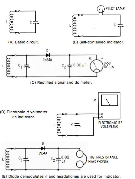
Fig. 3-1. Absorption wave meters. (A) Basic circuit. (B) Self-contained indicator.
(C) Rectified signal and dc meter. (D) Electronic rf voltmeter as indicator.
(E) Diode demodulates rf and headphones are used for indicator.
----------------------

Table 3-1. Wavemeter Coil Data
Variable Capacitor C = 140 pF
(A) 1. 1-3.8 MHz 72 turns No. 32 enameled wire closewound on 1" diameter plug-in form.
(B) 3.7-1 2.5 MHz 21 turns No. 22 enameled wire closewound on 1" diameter plug-in form.
(C) 12-39 MHz 6 turns No. 22 enameled wire on 1" diameter plug in form. Space to winding length of 3 ½ s".
(D) 37-1 50 MHz Hairpin loop of No. 16 bare copper wire.
Spacing of 1/2 " between straight sides of hairpin. Total length including bend: 2 inches.
--------------------------
In use, the wavemeter is loosely coupled to the unknown frequency source and tuned for resonance. For instance, the instrument may be held so that coil L is close to the output coil of a radio transmitter. Resonance can be indicated in various ways. When the circuit in Fig. 3-1A is used, for example, the unknown-signal source must have a current meter in its output stage (a plate milliammeter in a tube-type source, a collector milliammeter in a transistor-type source ) ; and the deflection of this meter will rise sharply as the wavemeter is tuned, the peak point of this rise indicating resonance. In the other arrangements, the wavemeter has a self-contained indicator. In Fig. 3-1B, this is a pilot lamp such as the 2-V, 60-mA Type 48.
The lamp glows brightest at resonance. This arrangement can be used only when the signal source supplies enough power to light the lamp. In Fig. 3-1C, a IN34A germanium diode (D) rectifies the rf energy and deflects a 0 to 50 dc microammeter (M) , the peak deflection of this meter indicating resonance.
In Fig. 3-1D, an electronic rf voltmeter (vtvm or tvm) is connected temporarily to the wavemeter and indicates resonance by peak deflection. In Fig. 3-IE, a 1N34A germanium diode (D) demodulates an amplitude-modulated unknown-frequency signal and applies the resulting audio voltage to high-resistance headphones. Here, resonance is indicated by the loudest sound.
Of these arrangements, the sharpest-tuning wave-meters are Fig. 3-1A, 3-1C, and 3-1D in that descending order. The least selective is Fig. 3-1B. In wave-meters containing an internal indicator (e.g., Fig. 3-1B, 3-1C, 3-1D, and 3-1E) , selectivity may be improved somewhat by tapping the indicator circuit down coil L to minimize loading of the tuned circuit. This then calls for a 3-terminal plug-in coil.
A wavemeter may be calibrated from an accurate rf oscillator or signal generator by coupling to that device and tuning the wavemeter to resonance successively at various frequencies of the generator. Use as many frequencies as it is possible to inscribe on the dial without crowding. Usually, a separate dial scale is required for each range of the wavemeter (A, B, C, and D in Table 3-1). The wavemeter shown in Fig. 3-1A has no indicator of its own. It may be connected in series with the "high" lead between the generator and an all-band radio receiver. The wavemeter will then act as a wavetrap, eliminating the signal from the receiver at resonance.
Professional, laboratory-type absorption wavemeters, once available with as good as 0.25 % accuracy, are no longer manufactured. Most simple absorption wavemeters today are homemade. The accuracy of these latter instruments depends upon (1) accuracy of original calibration, (2) resettability of dial, (3) readability of dial, (4) sharpness of resonance, and (5) freedom from body-capacitance effects. An accuracy of ±10 % would be considered good.
In spite of its shortcomings, the absorption wavemeter is very useful for determining approximate frequency. When very loosely coupled to a signal source, this instrument is insensitive to harmonics, unless the source is high powered, and therefore is not subject to confusion of frequencies. Moreover, the wavemeter is small (therefore easily hand-held and easily poked into close quarters ) and, in addition, it requires no power supply.
3.3 MICROWAVE WAVEMETER
This instrument (see Fig. 3-2 ) also called a microwave frequency meter, is somewhat similar in action to the absorption wavemeter described in Section 3.2. Employing neither inductance nor capacitance, it consists essentially of a high-Q resonant cavity tuned by means of a choke plunger. Microwave energy of unknown frequency is fed into the cavity via a waveguide fixture and out of the cavity via a similar fixture (another model of this instrument provides coaxial input and output). This arrangement allows the instrument to be inserted into a waveguide system or a coaxial system. The indicator (Fig. 3-2B ) contains a silicon diode (D) which rectifies the output of the wavemeter, a dc amplifier (AMP) which boosts the resulting dc output of the diode, and a dc milliammeter (M) which is deflected by the output of the amplifier. When the wavemeter is tuned to resonance, the deflection of the meter (M) dips sharply, and the unknown frequency then may be read directly in gigahertz from the spiral scale of the wavemeter dial.
The microwave wavemeter is supplied for a single frequency range with a frequency ratio varying from 1.42 :1 to 4.37 :1, depending upon range. A set of such instruments, such as the eight units in the Hewlett-Packard 530 group, gives a frequency coverage from 0.96 GHz to 40 GHz, with an overall accuracy of 0.065% to 0.17%, depending upon individual range.
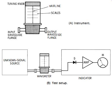
Fig. 3-2. Microwave wavemeter. (A) Instrument. (B) Test setup.
3.4 LECHER FRAME
For frequencies between 900 MHz and 15 GHz, measurements can be made in terms of the wavelength of standing waves set up along two parallel rods or wires by the unknown frequency source. The parallel-wire contrivance is termed a Lecher frame (see Fig. 3-3). The wires (No. 12 or heavier bare copper wire ) are each 2 feet long in their straight portion and are spaced about 1 inch apart. They are mounted solidly on standoff insulators on an insulating base and bent into a loop at one end for inductive coupling to the unknown-frequency source. The standing-wave detector is a radio-frequency meter consisting of a 1N21B silicon diode (D) and a 0 to 50 dc micro-ammeter (M). This detector is mounted on a simple sliding carriage so that it can be positioned at, and make contact with, any desired point along the length of the wires. If the signal source delivers at least 14 watt of rf power, the indicator can be simply a 2-V, 60-mA pilot lamp.
When rf energy from the signal source is coupled into the frame, standing waves appear along the wires. As the detector then is slid along the wires, meter M deflects upward to show high-voltage points (maxima ) in these waves and downward to show low-voltage points (minima). The operator carefully measures the distance, d, in centimeters, between any two successive maxima or successive minima. (This gives the wavelength of the unknown signal, in centimeters.) The unknown frequency then is calculated from this wavelength :
fx in MHz = 300,000/d
fx in GHz = 30/d
(Eq 3-1)
(Eq 3-2 )
Illustrative example : In a certain test with a Lecher frame, peak deflections are obtained at 10.5 cm and 16 cm along a scale permanently mounted on the frame. Calculate the frequency in megahertz.
Here, d = 16 - 10.5 = 5.5 cm. From Equation 3-1, f. = 300,000/5.5 = 54,545 MHz.
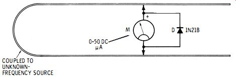
Fig. 3-3. Lecher frame.
In the first paragraph, 900 MHz is suggested as the lowest frequency for this method. This limit is based upon the 2-ft length recommended for the wires. Setups with longer wires or rods lack the mechanical stability required for the Lecher frame. Also, at lower frequencies (longer wavelengths ), the maxima and minima on the long wires become broad and hard to pinpoint. (In a 50-MHz system, the correct response points would be 19.7 feet apart. ) Accuracy of this method depends upon (1) accuracy of the centimeter measurement, (2) sharpness of maxima or minima indication, (3) extent of body capacitance, (4) looseness of coupling, and (5) care in the calculation. A value of 10ma is realistic.
3.5 SLOTTED LINE
At microwave frequencies, the slotted line, used primarily for other purposes, is a useful device for frequency measurement. Fig. 3-4 shows a test setup incorporating this device.
The slotted line is essentially a special section of coaxial line; as such, it consists of an outer metal cylinder and an inner, concentric metal rod. A lengthwise slot is cut in the outer cylinder (the device takes its name from this) , and a carriage is positioned to slide along the outside of this cylinder, carrying a metal probe which dips down into the space between the rod and the inner wall of the cylinder to sample the standing waves inside the cylinder. Inside the carriage, the probe is connected to a silicon point-contact diode (D). Although coaxial input and output coupling and a coaxial-type slotted line are shown in Fig. 3-4, slotted waveguides with waveguide-type coupling also are available.
When the slotted line is properly terminated and is adjusted by means of its tuning stub, rf energy from the unknown frequency signal source sets up a standing-wave pattern inside the cylinder. As the carriage is slid along, the probe passes through high-voltage points (maxima ) and low-voltage points (minima). These points are indicated by a detector consisting of diode D, the dc amplifier, and microammeter M; the meter deflects upward for maxima and downward for minima. A pointer on the carriage travels along a centimeter scale, allowing the operator to note the exact positions of these response points. From the distance between two successive maxima or two successive minima (which indicates the wavelength of the signal, in centimeters ), the unknown frequency can be calculated in megahertz with Equation 3-1 or in gigahertz with Equation 3-2.
The characteristic impedance of the slotted line is usually 50 ohms. Depending upon make and model, the scale is accurate to ±0.1 mm, and this is the accuracy with which the wavelength may be measured. Depending upon make and model, the slotted line may be used between 300 MHz and 8.2 GHz.
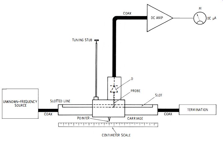
Fig. 3-4
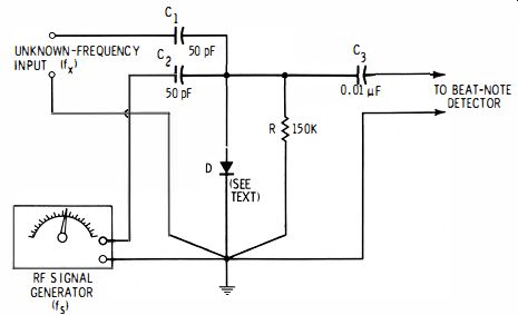
Fig. 3-5. Signal-generator method of rf measurement.
3.6 SIGNAL-GENERATOR METHOD
An accurate rf signal generator may be employed to check unknown frequencies by means of the beat-note method. Fig. 3-5 shows the test setup. In this arrangement, the signal of unknown frequency (fx) and the generator signal (fs) are applied simultaneously to a diode mixer circuit, and the resulting beat note between the two signals is delivered by the mixer to a beat-note detector. This detector can be an electronic ac voltmeter (vtvm or tvm) , high-impedance headphones (with or without an audio amplifier ), or an electronic audio-frequency meter (see Sections 2.4 and 2.5, Section 2). The generator is tuned to zero beat with the known signal, and at that point, fx is read directly from the generator tuning dial. For frequency measurement as far as 30 MHz, a germanium point contact diode, such as Type 1N34A, will be satisfactory for D in Fig. 3-5. At higher frequencies, a silicon point-contact diode, such as Type 1N21B, must be used.
Best results are obtained with a visual detector (electronic voltmeter or frequency meter ), since the relatively poor low-frequency response of headphones makes the exact point of zero beat hard to pinpoint by ear. In Fig. 3-5, the standard frequency source is variable, and the unknown-frequency source fixed, but the opposite arrangement also is feasible.
When the zero-beat point is sharply defined, the accuracy of this method can equal that of the signal generator.
3.7 HETERODYNE FREQUENCY METER
This instrument combines in one unit the separate sections used in the signal-generator method described in Section 3.6. Fig. 3-6 shows a functional block diagram of the conventional heterodyne frequency meter. In this arrangement, an internal, highly stable variable-frequency rf oscillator (B) with frequency-reading dial is tunable over a single fixed range (say, from 500 kHz to 1000 kHz) , and the output of this local oscillator is applied to a mixer (A) simultaneously with the signal of unknown frequency, fx. The resulting beat note is presented to the zero-beat detector and indicator (C).
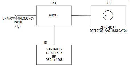
Fig. 3-6. Heterodyne frequency meter.
To check unknown frequency fx, the operator tunes the oscillator to zero-beat with the unknown and reads the frequency directly from the dial. This assumes, of course, that fx lies within the basic tuning range of the oscillator. But zero beat can be obtained also when fx is a harmonic or subharmonic of the oscillator setting. This situation allows frequencies both above and below the fundamental range of the oscillator to be measured. Thus, if the oscillator tunes from 500 kHz to 1000 kHz and zero beat occurs at 625 on the dial, fx could be 208.3 kHz, 312.5 kHz, 625 kHz, 1250 kHz, 1875 kHz, 2500 kHz, and so on. While it is this feature that gives the heterodyne frequency meter its wide range while employing only a single-range oscillator, it also invites error in frequency identification.
For this reason, the operator must determine whether he is zero-beating the fundamental, a harmonic, or a subharmonic.
With strong fx signals, an instrument with 500- to 1000-kHz basic tuning range can be useful from 50 kHz to 50 MHz.
Accuracy of the instrument depends upon that of the oscillator and may be as good as 2% of the indicated frequency at fundamentals and progressively worse as the harmonic number increases.
In another type of heterodyne frequency meter, the output of the mixer is an intermediate-frequency signal which is amplified by a sharp i-f amplifier and detected by a second detector. The dc output of the latter then actuates the indicating meter. When using this arrangement, the instrument is tuned for a peak deflection of the meter, instead of for a zero beat.
Some rf signal generators are equipped with a built-in mixer and headphone jack, to provide a heterodyne frequency meter for fx measurement. The several separate bands of the signal generator enable all frequency measurements over a wide span to be made on fundamental frequencies.
3.8 DIP METER
This small, hand-held instrument, also known as a grid-dip oscillator' in its tube version, is a standby with amateurs and experimenters. It is essentially a wide-band, variable-frequency rf oscillator with direct-reading dial and microammeter resonance indicator. Most dip meters have a special switch for disabling the internal power supply (while keeping the filament burning in the tube version ). This converts the instrument into a direct-reading absorption wavemeter (see Section 3.2 for use of the wavemeter). Resonance is indicated by peak deflection of the microammeter. The dip meter can also be used with power on to measure frequency by the zero-beat method if high-resistance magnetic headphones are plugged into the phone jack of the instrument. In this latter application, the instrument is operated in the same way as an absorption wavemeter, but the resonance indication is an audible indication of zero beat.
Depending upon make and model, dip meters-by employing a series of plug-in coils-cover the frequency span of 72 kHz to 300 MHz. Special types extend the frequency limit upward to 940 MHz and downward to 50 kHz. The dip meter is not intended to be a precision instrument, and most manufacturers give no accuracy figure for this device (those who do, specify ±3 %).
3.9 ANALOG-TYPE ELECTRONIC FREQUENCY METER
This type of instrument, which offers high input impedance, employs a D' Arsonval-type meter for direct indications of frequency and requires no tuning. It is described in sufficient detail in Section 2.4, Section 2 (which see).
This instrument originally was intended for audio-frequency measurements only, and 100 kHz was its maximum frequency.
Improved circuit design and modern manufacturing techniques, however, have greatly extended its frequency range.
One modern instrument (Hewlett-Packard Model 5210A) , for example, directly indicates frequencies from 3 Hz to 10 MHz in six bands : 0 to 100 Hz, 0 to 1 kHz, 0 to 10 kHz, 0 to 100 kHz, 0 to 1 MHz, and 0 to 10 MHz. The last three bands, of course, are of interest to the worker with radio frequencies. Accuracy is 1 % of reading from 10 % of full scale up.
While the analog-type frequency meter has been largely superseded by the digital type, the former is still valued in those applications in which a quick appraisal of up and down movements of frequency is desired (this is somewhat difficult to keep track of with the digital readout).
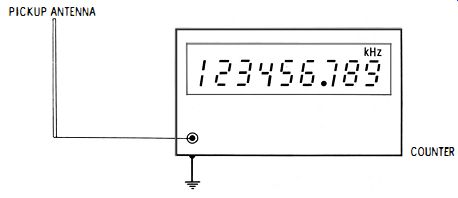
Fig. 3-7. Digital-type electronic frequency meter.
3.10 DIGITAL-TYPE ELECTRONIC FREQUENCY METER
The digital electronic counter is useful as a frequency meter at radio frequencies, as well as at audio frequencies where it is employed so widely. The general principles of this instrument are explained in Section 2.5, Section 2 (which see). Radio frequency energy from the unknown-frequency signal source may be introduced into the instrument either through a series capacitor or through a small pickup antenna plugged into the input receptacle (see Fig. 3-7) , or by means of a small pickup coil of a few turns.
Depending upon make and model, electronic counters give a direct display in either hertz, kilohertz, megahertz, or gigahertz up to 18 GHz and in 6, 8, 9, or 10 digits with the decimal point automatically placed. Input impedance is 50 ohms, 1 meg-ohm, or both. Sensitivity ranges from 10 mV to 35 mV rms sine wave, accuracy is ±1 digit ± the time-base error.
The digital counter has become increasingly popular as a frequency meter because its operation is instant and automatic and because it can display a number of digits for the close reading of frequency.
3.11 WAVE ANALYZER
The wave analyzer is an instrument intended primarily for the evaluation of a signal and its various harmonics. However, since it is continuously tunable with a dial reading directly in frequency units, this instrument is useful also as a frequency meter. The wave analyzer is tuned simply for peak deflection of its self-contained electronic voltmeter, and the frequency then is read directly from the dial. The operating principle of the wave analyzer is explained in sufficient detail in Section 2.7 A, Section 2 (which see). The conventional wave analyzer is designed for the 20-Hz to 20-kHz range. However, the operation of some modern models extends high into the radio-frequency spectrum. A tuning range of 1 kHz to 18 MHz in 18 overlapping bands thus is provided by one model (Hewlett-Packard 312A) with digital electronic readout (accuracy is ±10 Hz + the time-base accuracy). Within its range, the wave analyzer can be used as a sharp-tuning continuously variable frequency meter which will show not only the unknown radio frequency, but also the signal amplitude. It will also, by its nature, evaluate each of the harmonics of the signal.
3.12 OSCILLOSCOPE METHODS
High-frequency oscilloscopes can be used to some extent for the measurement of radio frequency. The principal methods are described below.
A. Oscilloscope having calibrated time base.
Modern factory-built oscilloscopes and some kit-type oscilloscopes, as well, come equipped with a calibrated horizontal sweep system which can be read directly in seconds, milliseconds, microseconds, or nanoseconds percentimeter or per screen division from the settings of front-panel selectors and multipliers. These instruments provide a number of ranges, such as 10 ns/div, 0.2 f-ts/cm, 100 ms/cm, and 1 s/div. It is not uncommon for one instrument to provide as many as 20 selectable rates. Accuracy is usually ±3% to ±5%. The period (t) of 1 cycle of an unknown frequency is easily found by measuring the time width of this cycle along the horizontal axis, and from this, the frequency is calculated : fx = lit (Eq 3-3 ) where, fx is in hertz, t is in seconds.
Illustrative example : When the sweep rate of a certain oscilloscope is adjusted to 100 ns/cm, 1 stationary cycle of the applied unknown-frequency signal is 3.3 cm wide. Calculate the frequency in megahertz.
Here t = 3.3 (100) ns = 330 ns = 3.3 X 10^-7 s.
From Equation 3-3, f. = 1/3.3 X 10^-7 = 3.03 X 10^10 Hz = 3.03 MHz.
Some sophisticated, laboratory-type oscilloscopes give a direct, automatic readout of lit, i.e., of frequency, thus obviating the need for any calculations.
B. Use of Lissajous figures
When the horizontal channel, as well as the vertical channel, of an oscilloscope will handle radio-frequency signals, a radio-frequency signal generator or frequency standard may be employed to identify unknown frequencies by using Lissajous figures. The accuracy of this method can equal that of the generator.
Except for the precautions which apply to any rf test (see Section 3.1) and for the higher frequencies involved, the techniques for Lissajous figures at radio frequencies are the same as for audio frequencies. These are explained in Section 2.6B, Section 2, and the reader is referred to that section for instructions and sample patterns.
C. Use of individually calibrated screen
Except for the precautions which apply to any rf test (see Section 3.1) and for the higher frequencies involved, the procedure for radio-frequency checking with an individually calibrated screen is the same as for audio frequencies. The technique is explained in Section 2.6F, Section 2, and the reader is referred to that section for instructions and sample patterns.
D. Use of dual-trace oscilloscope Except for the precautions which apply to any rf test (see Section 3.1 ) and for the higher frequencies involved, the procedure for radio-frequency checking with a dual-trace oscilloscope is the same as for audio frequencies. The technique is explained in Section 2.6F, Section 2, and the reader is referred to that section for instructions and a sample pattern.
3.13 RADIO RECEIVER
An all-band radio receiver is useful as an emergency, widerange radio-frequency meter. A communications-type receiver may be tuned for peak deflection of its self-contained S meter; in other receivers, an electronic dc voltmeter connected temporarily between the agc bus and ground will serve as the tuning indicator. For most reliable operation, the receiver must be loosely coupled to the unknown-frequency signal source.
Except for communications receivers of older vintage, frequencies may be read directly from the tuning dial. The accuracy of a receiver employed as a frequency meter depends upon (1) accuracy of the original calibration, (2) freedom from drift, (3) readability of dial, and (4) resettability of dial.
From 1% to 2% of indicated frequency would be considered excellent. Some communications receivers are equipped with a self-contained frequency spotter (e.g. , a 100-kHz crystal oscillator ) having harmonics to provide check points for periodic recalibration of the dial. With this refinement, the receiver can be recalibrated prior to each use as a frequency meter and can offer enhanced accuracy.
In the use of a superheterodyne receiver as a frequency meter, care must be taken to distinguish between images and real signals. The most satisfactory receiver for this application will, of course, be one having an excellent signal-to-image ratio. Care must also be taken against interfering signals from radio and tv stations (see Section 3.1F).
3.14 FIELD-STRENGTH METER
Like the radio receiver (Section 3.13) , a frequency-calibrated field-strength meter also can be used as a continuously tunable, direct-reading radio-frequency meter ; and, like the receiver, the field-strength meter employs a superheterodyne circuit for improved sensitivity and selectivity. Peak deflection of the self-contained microammeter of this instrument indicates exact tuning to a signal, and additionally this meter reads directly in volts, millivolts, and microvolts.
Conventional field-strength meters cover the ranges normally offered by general-coverage communications receivers, i.e., 500 kHz to 50 MHz, and some tune as low as 100 kHz.
Accuracy is from ±1 % to ±3 % of indicated frequency. Some special field-strength meters cover television-channel frequencies only and are step-tuned, not continuously tunable.
Radio-frequency energy may be coupled into the field strength meter via capacitance coupling, antenna pickup, or low-impedance transmission line. Some instruments make provision for all of these.
3.15 FREQUENCY SPOTTER
A frequency spotter is a single-frequency rf oscillator (usually of the crystal type ) whose fundamental frequency is so chosen that its harmonics provide spot frequencies at convenient test points throughout a substantial portion of the radio-frequency spectrum. Thus, a 100-kHz oscillator may provide such check points every 100 kHz apart, from 100 kHz to 30 or 40 MHz. If the oscillator is closely stabilized, these spot frequencies are very reliable.
The spot frequencies may be monitored with a receiver (see Section 3.13), mixer (Section 3.6) , heterodyne frequency meter (Section 3.7) , or hf wave analyzer (Section 3.11 ). The fundamental frequencies commonly selected for frequency spotters are 50 kHz, 100 kHz, 1000 kHz, and 5 MHz. Some communications-type radio receivers are equipped with a self-contained 100-kHz crystal oscillator for frequency spotting.
The successive harmonics from a frequency spotter diminish in intensity. The highest spot frequency that has useful amplitude depends upon oscillator power output and the amount of intentional distortion in the signal. (A sine-wave signal has few harmonics, in a practical sense, and is of no value in this application.) In general, tube-type oscillators-since they operate at higher dc voltage than do transistor oscillators-give useful harmonics farther into the spectrum.
It should be noted that the frequency spotter is not itself a frequency-measuring device, but rather a generator of dependable signals which may be used as the standard-frequency (fs) source in test setups. When operation of this device is closely stabilized to minimize frequency shift due to variations in voltage, temperature, humidity, and other parameters, the frequency spotter becomes a frequency standard and as such is discussed in the next Section.