SIGNAL TRACING IN CONTROL CIRCUITS [Servicing by Signal Tracing (1939)]

AUTOMATIC volume control, generally called "ave," has become an integral part of practically all commercial radio receivers. The few modern receivers which are not so equipped are mainly small tuned r-f sets, employing not more than three or four tubes.

It is easy to see why automatic volume control has been so universally adopted. The signal strength of broadcast programs in any one radio receiver installation may vary over an extremely wide range as great as one million to one. A nearby powerful station may provide a signal as strong as one volt across the antenna while another station, weaker and remote from the receiver, may supply a signal of only two or three microvolts.

Even strong signals sometimes fade, due to changes in the transmitting medium between the transmitter and the receiver, so that the received signal fluctuates. These various influences, up to the time automatic volume control was introduced, represented some of the objectionable characteristics of broadcast reception.

Automatic volume control controls sensitivity by making the gain of the receiver lower for strong signals than for weak ones.

This is done automatically and in a perfect avc system only as much reduction in gain takes place as is required to provide a uniformly strong signal to the detector in the receiver.

If we tune the receiver from one station to another which is ten times as strong, the sensitivity of the receiver is automatically reduced to about one-tenth of what it was for the first station.

Therefore the signal which reaches the detector is of substantially the same strength for both stations. If there were no avc in the receiver, the stronger signal would produce a much louder sound from the speaker, or, if the speaker were already working at full volume, one or more of the tubes in the receiver would become overloaded and reception would be weak and distorted. Through the use of ave, such troubles are avoided. One can tune from one station to another which is weaker or stronger without bothering to readjust the volume control to give the desired sound volume. And the possibility of "blasting" when passing from a weak station to a stronger one is eliminated.

Automatic volume control also increases the sensitivity of the receiver when the set is tuned from a strong signal to a weaker one. Thus it is possible to rotate the tuning dial over its range without. continually readjusting the volume control to avoid passing a desired weak station which otherwise might not be heard.

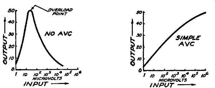
Figs. 7-1 (left), 7-2 (right). The variation in output of a receiver with out avc for different values of input signal is shown at the left. When avc is used, no overloading takes place on strong signals.

This increase in sensitivity, under these conditions, does not mean that additional amplification is put into the receiver; it means that more of the amplification of which the receiver is capable is being utilized. Receivers employing automatic volume control usually operate at the maximum possible sensitivity of which they are capable when no signal at all is being received. Then, as soon as any signal which the receiver is able to detect is received, the avc starts to function.

No avc system is perfect. If it were, then every signal within the sensitivity range of the receiver would be of precisely the same strength at the detector. However, a very substantial degree of uniformity of signal strength is realized through its use. With even a simple avc system, a change in input signal from 10 microvolts to one volt changes the receiver output from 10 units to 50 units. In other words, a change of 100,000 to one in the input signal level changes the output signal level in the ratio of only 5 to 1.

The action of a simple avc system is shown graphically in Fig. 7-2. Note that the curve climbs uniformly and gradually tapers off. Comparing Fig. 7-2 with Fig. 7-1, it is significant to note …

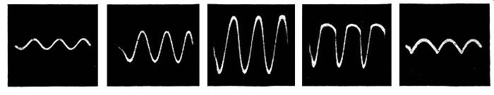
Figs. 7-3 to 7-7, left to right. These oscillograms show how the output of a receiver without avc changes as the input signal is increased.

... that Fig. 7-2 shows no overload point. While the receiver with out ave, shown in Fig. 7-1, overloads considerably with an input signal of less than 100 microvolts, the receiver equipped with simple avc does not overload even when the input signal is as …

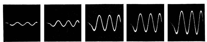
Figs. 7-8 to 7-12, left to right. These oscillograms show how the avc action prevents overloading as the input signal is increased.

... much as 1 volt. This is also demonstrated by comparing the waveforms of the output signals in Figs. 7-3 to 7-7 inclusive with those shown in Figs. 7-8 to 7-12 inclusive. The excellent wave form of the latter, even at high signal levels, shows that no distortion results at any signal level while in Fig. 7-6, without ave, the output is already badly distorted when the input signal is 200 microvolts. These figures do not represent the performance of any one specific receiver, but rather are simple illustrations of the action of a receiver without ave.

Delayed AVC

A close examination of Figs. 7-1 and 7-2 shows that a receiver which is equipped with simple avc has lower sensitivity for very small input signals than one without ave. The reason for this is that simple avc acts to cut down the sensitivity of a receiver as soon as a signal is received and this happens no matter how weak the signal may be. This is a disadvantage, since the maximum sensitivity of the receiver is required when weak signals are tuned in. This makes very weak signals difficult to receive properly because, during the time when the maximum sensitivity is needed, the action of the avc lowers the sensitivity.

To enable better reception of very weak signals, the type of circuit known as "delayed ave" was introduced. The improved performance made possible with this type of circuit is due to the fact that the application of avc action is delayed until the signal strength reaches a certain predetermined value. Practically, this means that for very weak signals there is no avc action.

A performance curve of a receiver equipped with delayed avc is shown in Fig. 7-13. You will note that for small values of …

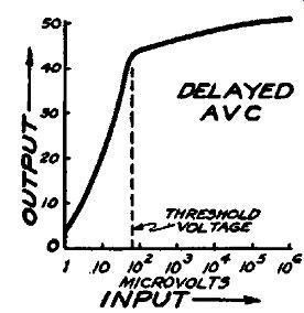
FIG. 7-13. In delayed avc circuits, the application of the control voltage is delayed until a minimum value of input signal is reached. Beyond this threshold voltage, the avc action keeps the output al most constant.

… input signal, up to about 60 microvolts, the operation of the receiver is similar to that of the one shown in Fig. 7-1. That is, the output is proportional to the input for signal inputs up to this level. In other words, the receiver performs for weak signals just as if it were not equipped with ave. Yet, when the signal level exceeds 60 microvolts the avc action begins to "take hold" and the control effect for strong signals, where it is most needed, is present.

Quiet AVC

We mentioned previously that receiver sensitivity is greatest when no signal is being received, because the avc action cannot take place until a signal reaches the detector or avc tube. Now, in actual operation of a receiver, as we rotate the dial over the tuning range, there are some points where signals are present and others where signals are not received. At these points where no signal is being received, the sensitivity of the receiver is greatest.

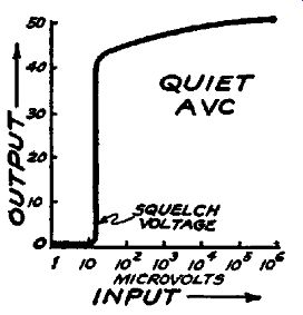
Fig. 7-14. In quiet avc or noise suppression circuits the output is zero for small values of input signal. Above the squelch voltage point, the normal avc action keeps the output essentially constant.

Yet a certain amount of electrical noise is always present in the antenna system and consequently we find that the maximum sensitivity of the receiver again is available when it is undesirable, i. e., when only noise is present. This is naturally very annoying so a means for overcoming this fault also has been devised. This means is known as quiet avc or "q_ave."

Quiet avc functions to reduce the sensitivity of the receiver until the signal reaches a certain predetermined level. Since the noise level in any given location varies from day to day and often from hour to hour, provision is made to adjust the level at which the signal will be received. In other words, by this method we can adjust the receiver so as to receive a weak signal with noise, if desired, or to reduce the sensitivity so that the signal must be stronger than the noise before it will be heard.

The relation between the output signal and the received signal is shown in Fig. 7-14. In contrast to Figs. 7-1 and 7-2, Fig. 7-14 shows the relation between the receiver output signal and the received signal rather than the second detector output and the received signal, as in Figs. 7-1 and 7-2. The reason for this is that in q_avc systems, which are also known as noise-suppression and squelch circuits, the action of the avc system is to block one of the audio tubes during the time that the received signal is below a predetermined level and to open the system when the received signal is of sufficient intensity. This is one method; others will be discussed later.

If you will examine Fig. 7-14, you will note that there is no output from the receiver over a certain range of input signal levels--from zero input up to a certain predetermined value. It is during this time that the audio system is blocked by the control circuit. Then, if the receiver is tuned to some station which is received with an intensity equal to or greater than the critical value, generally known as the squelch voltage, the audio system is unlocked and normal avc operation is restored. It is because of this steep rise in the output that receivers equipped with q_avc are silent during tuning and then, when the proper signal is tuned in, the output signal suddenly appears.

These are the fundamental properties of the three principal types of avc systems. What we have tried to do up to this point is to develop a general acquaintance with the main features of these systems and to show how each works toward the ultimate goal of ave. The various circuits utilized to accomplish the results described are basically the same but contain extensive modifications which we will discuss from the signal-tracing stand point, because automatic volume control, like many other forms of automatic control of receivers, is operated by and for the signal.

We stated that automatic volume control, as the term is generally understood, is really the control of the sensitivity of the receiver ahead of the second detector tube-and that this control of sensitivity depends upon the intensity of the received signal.

Now in order to control the sensitivity of the receiver automatically, it is necessary to control the amount of gain or amplification available in the r-f and i-f amplifiers. But in order to understand how the amplification of these stages is controlled, it is essential to comprehend the manner in which the amplifying properties of tubes can be varied.

Controlling Gain

In avc systems, varying the control-grid bias is used as a means of varying the mutual conductance and consequently the amplifying properties of tubes in the r-f and i-f amplifiers. Since the sensitivity of the receiver is dependent upon the amount of gain or amplification in the r-f and i-f amplifying stages, by varying the mutual conductance of the tubes in these stages, avc controls the sensitivity of a receiver.

The manner in which the control-grid voltage changes the plate current and gain in any tube depends upon a number of different factors, primarily the design of the tube. However, irrespective of design, one condition exists in general-an increase of the negative bias applied to the control grid reduces the plate current and likewise reduces the gain or amplification available with the stage. If we express this condition in relation to the sensitivity of the receiver, rather than in terms of gain or amplification, it means that an increase in the negative control-grid bias applied to the r-f and i-f tubes in a receiver reduces the sensitivity of the complete system.

Not all tubes are equally suitable for use in amplifiers which are controlled by ave. With some tubes, the reduction of sensitivity which occurs as a result of increasing negative bias on the control grid is so abrupt that the controlled tubes cease to function as amplifiers and act as rectifiers. Then distortion results.

In Fig. 7-15, for instance, curve A represents the variation in mutual conductance which takes place with a "sharp-cut-off" tube, such as the 24, 57, 6C6, 6J7, etc. Note that the mutual conductance drops to zero for a very small value of grid voltage, approximately 7 volts. The amount of signal voltage permissible in these tubes is definitely limited by the very low bias voltage.

Consequently strong signals overload the tube. Then when the bias voltage is applied as a control voltage, it is very critical and its range of operation is extremely limited. To reduce the sensitivity of a very strong signal to the required level a fairly high bias is needed. This results in operation near cut-off and rectification occurs. The result is distortion and cross-modulation, which is the "riding through" of an undesired station on the carrier of a desired station. In r-f amplifiers, increase of the control-grid bias causes distortion of the modulated wave envelope and this, in turn, causes a distorted audio output.

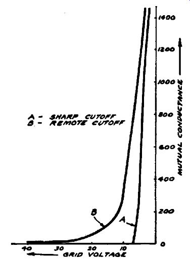
Fig. 7-15. The variation in the mutual conductance of sharp cut-off and remote cut off tubes. The gradual cut-off shown in curve B makes the remote cut-off pentode suit able for use in receivers equipped with avc.

Curve B in Fig. 7-15 represents the characteristics of a remote cut-off tube, such as the 35, 58, 6D6, 6K7, etc. Note that the change in gain as a result of increasing control-grid bias is very gradual and extends over a very wide range, cut-off not appearing until approximately -40 volts bias has been applied. Operation without rectification due to overload is therefore possible even with very strong input signals. Such is the type of tube used in the r-f and i-f amplifiers of receivers equipped with avc.

Let us now consider the characteristics of the control voltage which is utilized to reduce the gain depending upon the strength of the signal being received. It stands to reason that since it is to act as a bias voltage it must have d-c characteristics, yet since it is to vary as the incoming signal varies in strength, it must be produced as the result of an applied signal. Since the signal is an alternating current, some form of rectification is therefore necessary.

As a high control voltage is often necessary when the incoming signal is very strong, the rectifier for the avc voltage is usually placed at a point in the circuit where the signal voltage is strong est. This point is in the output circuit of the last i-f stage of a superheterodyne receiver, since the signal must pass through all the amplifying stages before it reaches this point. Since rectification is also necessary for detection, both these functions are frequently combined.

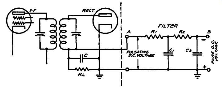
Fig. 7-16. A typical diode rectifier and filter. The filter circuit shown at the right removes the audio component from the avc voltage.

In the section on detectors we saw that the diode provides a convenient means for obtaining a d-c voltage which is proportional to the strength of the signal. Since the action which takes place in a rectifier for avc purposes is essentially the same as in a detector, we need not repeat the discussion of diode rectifiers in this section. Referring to Fig. 7-16, which shows a typical diode rectifier and filter which are used to operate an avc system, we note that this circuit is in many respects similar to Fig. 3-4. Thus the modulated input produces a d-c voltage at point A which is proportional to the strength of the carrier and an audio voltage which is dependent upon both the strength of the carrier and the percentage of modulation. In the section on detection, we were primarily interested in the audio part of the voltage across the diode load, whereas in the present section we are interested in the d-c voltage across the diode load.

We know that the purpose of this d-c voltage is to function as a control-grid bias. This means that the circuits to which this voltage is applied consume no direct current. Consequently, no direct current flows through resistors R1 and R2; this means that there is no d-c voltage drop across R1 and R2. Therefore, the d-c voltage at point B is the same as that at point A. The fact that no d-c flows in this circuit accounts for the use of high resistance instead of chokes, which are needed to reduce the d-c resistance in power supply circuits where d-c also flows in the filter circuit.

In the case of the audio or a-c component, the action is some what more complex. The capacities of C1 and C2 are so chosen that they offer a low impedance to the flow of alternating Currents of low frequency. This means that only a very small part of the total a-c voltage will be developed across the first filter condenser, C1, because of its relatively low impedance with respect to the first filter resistance, R1. The a-c voltage is further reduced in the same way by the R2-C2 combination, which forms the second section of the filter, so that the output of the filter is essentially a pure d-c voltage.

The reduction in a-c voltage by means of this filter depends upon the frequency of the audio signal. For higher frequencies, the filter action will be more effective; for lower frequencies, it will be proportionately less. Since, in broadcasting, frequencies below 100 cycles are often present, it is important that the avc filter be effective even at such low frequencies. Since increasing the values of C1 and C2 would improve the filter action, why not do so? The answer is that it takes a certain amount of time for a condenser to charge and discharge when there is resistance in the circuit. This is described by the "time constant" which is the actual time in seconds required for a given condenser to receive 63 percent of its final charge; its value is equal to the product of the total capacity in the circuit times the total resistance in series with the capacity. In a circuit composed of a 1-megohm resistor in series with a 1-mf condenser., the time constant is one second.

Once the condenser has received a charge, it takes an equal amount of time for its voltage to drop to 37 percent of its original value.

What effect does this time constant of the avc circuit have on the operation of the circuit? Simply this--when we tune from a strong signal to a weak one, it is important that the avc voltage change as rapidly as one rotates the tuning dial, otherwise the high avc voltage which is developed for the strong signal will "hang on" and temporarily reduce the sensitivity of the receiver when the tuning point for the weak signal is reached. Then the signal may not be heard. Also, in tuning from a weak signal to a much stronger one, if the avc voltage takes too long to reach its proper value, the strong signal will blast and then gradually fade as the avc voltage approaches its maximum and therefore reduces the sensitivity of the receiver. The final result is that the choice of values for the resistors and condensers in an avc circuit is a compromise, and the values chosen are those which will give satisfactory filter action and yet keep the time constant low enough. These values, in commercial broadcast receivers, are generally chosen so that the time constant is about 1/10 th second. In making replacements of defective condensers in avc circuits, it is important to realize this limitation regarding the size of the replacement condenser. Don't use a larger value of capacitance than is called for on the schematic on the theory that too much capacity is always better. Replace with the identical value specified by the manufacturer.

Basic Control Circuit

While there are a great many types of avc circuits, all operate upon the same basic principle-the incoming signal is used to actuate a device which develops a d-c voltage to be used for control purposes. The manner in which this is done has been discussed in detail so that, no matter how complex the circuit may be, its fundamental operation may be readily understood.

Since all such automatic control circuits are actuated by the signal, it follows that tracing this signal is necessary in any complete check of the performance of such circuits. Let us first consider a simple avc circuit and trace the signal from point to point in the circuit.

The diagram, Fig. 7-17, can be considered to represent an i-f stage and avc rectifier of a superheterodyne receiver. Let us assume that a modulated signal is being applied to the input terminals of this receiver and has been traced, stage by stage, to the avc rectifier. If the intermediate frequency employed in the i-f amplifier is 465 khz, then a strong, modulated 465 -khz signal should be present at point 1, the avc diode plate. At point 1, if the by-pass condenser C is functioning, this 465 -khz signal should be reduced to a very low value. But since the signal is modulated, a strong audio voltage should be present at point 2. We know from our previous study of avc filter circuits that the purpose of R1-C1 and R2-C2 is to filter out the audio signal voltage which is normally present at point 2. So we trace this audio signal to point 3 and compare the value of the audio signal voltage found at this point with that at point S. It should be very much lower at point e and in fact for ordinary modulating frequencies its value will be negligibly small. At point 4, only a bare trace of audio signal will be left so that the control voltage which is applied to the grid of the i-f amplifier tube (point 5) is essentially pure d.c. We need not check the audio signal at point 5 since no additional filtering of the control voltage is contributed by the i-f transformer tuned circuit.

So far we have discussed signal tracing in this avc circuit on the assumption that the circuit is performing normally. Also we have confined our discussion to the modulated signal which actuates the avc rectifier. Before considering the resulting d-c control voltage, let us see how faults in the circuit are revealed by the procedure just described.

The 465 -khz signal voltage at point 1 is normally about one-half to one-third that present at point 6, the plate of the last i-f tube.

If there is a short or open circuit anywhere in the circuit from the plate to the cathode of the avc rectifier, this signal voltage will be greatly reduced. If condenser C should become shorted, or either R1 or RL should become grounded at point 2, the load on the tuned circuit would become extremely heavy; consequently the signal voltage at the diode plate would be greatly reduced.

Similarly, shorted turns in L3, which might not be revealed in ordinary resistance testing, would reduce the signal voltage at point 1.

An open circuit, whether in R_L, C, L_3, or its trimmer condenser, would drop the applied signal voltage at the diode plate to a very low value or eliminate it completely, depending upon the component affected. If C were open, for instance, the signal volt age would not be by-passed around R_L, consequently the signal voltage measured between the plate and cathode of the diode would be dropped by the resistance RL, which then would be in series with the tuned circuit. An open circuit in the trimmer condenser across LS would obviously make it impossible to tune LS to resonance; therefore the maximum voltage which the circuit was capable of producing would not be applied to the diode.

While an open or short circuit in the filter system at points 3 and 4 will have practically no effect upon the signal voltage at points 1 and S, ineffective filtering will be revealed by signal tests at points 3 and 4.

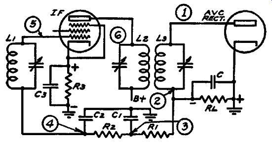
FIG. 7-17. An i-f stage and avc rectifier in a superheterodyne receiver. The avc voltage produced by the rectifier is applied to the grid of the i-f tube to control its gain.

If C1 is open, the audio signal at point 3 will not be by-passed and the actual signal voltage at this point will then depend upon the ratio of R2 to R1 plus R2. Assuming that R2 is 0.5 megohm and Rt is 1 megohm, the ratio of R2 to R3 plus R2 is equal to 0.5/1.5 or 1/3. So, when C1 is open, the audio signal voltage at point 3 with the filter resistors shown will be one-third that at point 2. Yet we know that the audio signal voltage at point S should be negligibly small and far less than that at point 2 when the filter circuit is performing properly. In. practical trouble-shooting, an approximate idea of what the signal voltages at these points should be is all that is necessary.

So far we have considered only the signal voltage in various parts of the avc system. We know, from our previous analysis of avc circuits, that a rectified d-c voltage should result from the signal applied to the avc diode, and that this resulting d-c voltage should he the same at points 1, 2, 3, 4 and 5. Leakage, short circuits or open circuits at points 3, 4 and 5 will affect the voltage readings at these points and consequently the avc action. Such troubles are localized by comparing the voltage readings at these points with that at point 1 or point 2.

A strong signal voltage should be present at the diode plate when making d-c voltage measurements in avc circuits. Then the rectified d-c voltage may be checked either at point 1 or point 2.

Since there is no appreciable voltage drop across the coil L3, the reading at point 1 should be the same as that at point 2, so either of these points can be checked to determine a reference voltage reading for comparison with the readings obtained at other points in the circuit.

Let us suppose that C1 is leaky. Then some of the direct current 1n this filter circuit will pass through this resistance leak to ground and the voltage at point 3 therefore will not be the same as that at point 2. If, for instance, R1 is 1 megohm and the resistance of C1, due to leakage, is also 1 megohm, the effect is similar to that which would occur if two 1-megohm resistors were joined together and shunted across RL. They would form a voltage divider, and since both resistors are of equal value, the voltage at the junction of these two resistors would be one-half the total voltage across R_L. In the diagram, this would mean that the d-c voltage at point 3 would be one-half that at point 2.

Suppose that Rt is open; then no d-c voltage (except the contact potential at the i-f grid) will be present at point 3, though the voltage will be normal at point 2. A decrease in resistance of R1, if of sufficient magnitude to affect appreciably the filter action would be revealed through signal tracing, though it would not affect the d-c voltage at this point. The same applies if a short-circuit exists between points 2 and 3. The second section of the filter can be checked in the same manner at point 4.

We have pointed out that normally no d-c flows in the avc filter circuit. However, in making voltage measurements some current must flow through the input resistance of the test instrument unless a type of voltmeter is used which consumes no current whatsoever. Since the types of meters generally employed in service work usually place some load on the circuit under test, the readings obtained are not the true voltages present at each test point. Just how much error is introduced by the loading effect of the voltmeter depends upon its input resistance for the range being used.

To keep this error to a minimum, the input resistance of the voltmeter must be very high in comparison with the resistance of the circuit under test. Since all avc filter circuits are of high resistance, the instrument used for measuring d-c voltages in such circuits must have an input resistance of about 10 megohms or higher.

When measurements of d-c voltages are made at points where an r-f signal is present, it is not enough that the input resistance of the voltmeter be high. In addition, care must be taken to prevent detuning of the circuit. This can be done provided the measurements are made with a special isolating probe as described in Section 12 and shown in Fig. 12-3. This probe must of course be used with a suitable high resistance voltmeter.

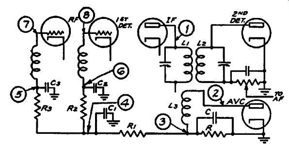
Fig. 7-18. An avc system in which a separate rectifier tube is used to produce the control voltage. Both the r-f and 1st-detector stages are controlled.

Fig. 7-18 shows an avc circuit in which the avc rectifier is inductively coupled to the primary of the last i-f transformer. L3 is untuned, but due to its close coupling to L1 a portion of the i-f signal is transferred to the avc rectifier and applied to the diode. The avc voltage is developed across the load resistor R and is applied to the r-f and first detector tubes through the common filter R1-C1 and the individual grid filters R3-C3 and R2-C2.

Testing of this circuit follows along the same lines as that described previously. The i-f signal is first checked at point 1 then at point 2, to make certain that the signal is being transferred to the diode circuit .. Since the avc rectifier is used only for avc operation and not as a detector, there is no need to keep C small enough in capacity to avoid by-passing audio frequencies.

So if C is of the order of 0.01 to 0.1 u-f, little a-f voltage should be found at point 3. If, however, C is 0.0005 u-f or lower in capacity, the a-f signal will be found and traced for proper filtering through the filter circuits by testing at points 4, 5 and 6. The control voltage may be tested at points 2 or 3 and the resulting voltage reading compared with that secured at any of the numbered points in the balance of the avc circuit.

Another form of simple avc circuit is shown in Fig. 7-19. As shown, a triode instead of a diode is employed as the avc tube.

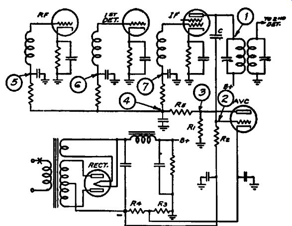
Fig. 7-19. An avc circuit in which a. triode is used as the avc rectifier. Note the distribution of the d-c voltages.

The i-f signal voltage is fed from the plate of the last i-f tube by means of the coupling condenser C to the grid of the avc rectifier. This signal voltage causes a change in the plate current of the avc tube and therefore a change in the voltage drop across R1. Though Rt returns to ground, the cathode and grid of the avc tube are both negative with respect to ground; the plate of the avc tube is accordingly positive with respect to its cathode.

The grid of the avc tube is connected to a point in the power supply system which is highly negative with respect to the cathode so that no plate current flows when no signal voltage is applied to point 2. Then, since no current flows through R1, there is no voltage drop across it and therefore point 3 is at ground potential. When an i-f signal is applied to point 2, the grid of the avc tube swings in a positive direction on the positive half of the signal wave, causing plate current to flow through R1 and making point 3 negative with respect to ground.

In signal tracing, the usual procedure of feeding a modulated signal to the receiver input terminals is followed. This signal is checked at point t and the signal strength noted. The presence of the i-f signal at point 2 shows that the coupling condenser C is performing its function. Note that the i-f is not by-passed at this point, nor at point 3. The a-f signal may be checked at point S and the functioning of the avc filter determined by noting the a-f signal attenuation at point 4. Individual decoupling and avc filtering is provided for each tube under avc control. The action of these filters is checked by testing at points 5, 6, and 7.

In checking the d-c voltages, a negative voltage reading at point 2 will of course be normal even when no signal is applied to the grid of the avc tube; then it should become increasingly negative as the signal voltage is raised; the actual d-c voltages at points 3, 4 and 5 should be the same at point 2. This control voltage can be traced through the numbered points in the avc system in the manner described before.

Delayed A VC Systems

We have discussed earlier in this section the limitations of simple avc systems and the reasons why delayed avc systems are sometimes used. We know, then, that by delaying the application of the avc voltage until the signal reaches a certain strength the sensitivity of the receiver to weak signals is increased. Let us now consider a few representative circuits and see how this is accomplished and how faults in such circuits are revealed by signal tracing.

In all delayed avc systems, a separate tube or a separate section of a double tube is required to obtain the delay action. The reason for this is obvious: if a combination detector and avc tube were used and the avc voltage were taken from the common diode load resistor across which the a-f voltage was being developed, any means which would render the avc action inoperative until a certain signal level were reached would likewise eliminate the desired a-f signal until it reached the same intensity.

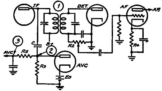
Fig. 7-20. A typical delayed avc circuit. The delay voltage E_b prevents the avc diode from rectifying the signal until the peak signal exceeds the delay voltage.

In delayed avc systems, no current flows in the diode circuit until the signal reaches the desired level. Consequently some means must be incorporated in the circuit to prevent current flowing through the diode load until this point is reached. One method of doing this is to apply a positive bias to the diode cathode. This is equivalent to applying a negative bias to the diode plate, since the cathode is the reference point in all considerations of tube operating voltages.

Fig. 7-20 shows a typical delayed avc circuit. The delay volt age is supplied by the battery En which biases the cathode of the avc tube. Since the plate is negative with respect to the cathode, no current flows in the diode circuit and therefore there is no voltage drop across RS. However, when an i-f signal reaches a peak value in excess of the biasing delay voltage, current flows in the diode circuit and therefore point 2 becomes negative with respect to ground. This forms the control voltage which serves to actuate the controlled tubes.

Signal tracing follows along the same lines as that for any type of simple avc system. Since the resistor RS is unby-passed, both i-f and a-f signals will be present across R3. The filter action is checked at point 3 and as well as the corresponding grid return points of tubes under control.

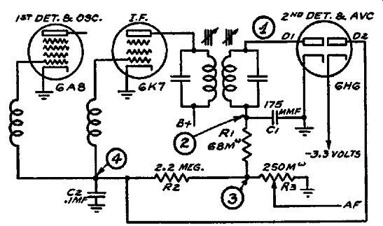
FIG. 7-21. In addition to the avc action being delayed, the cathodes of the controlled tubes are grounded and the minimum bias is obtained through the use of the auxiliary diode D2.

Fig. 7-21 shows another method of accomplishing delayed avc action. The delay action is obtained by shunting a second diode across the avc network at point 4. The cathode of this second diode is biased negative with respect to the plate, which is another way of saying that the plate is positive with respect to the cathode. Accordingly, the second diode draws current and will continue to do so until sufficient negative voltage is applied to the plate to exceed that of the cathode. Since the cathode voltage is -3.3 volts, this means that the voltage applied to the plate must exceed -3.3 volts before the diode ceases to draw current. As long as the plate voltage on this diode is less than -3.3 volts.

it forms a low-resistance load across the avc network because of its connection to point 4, Therefore, until sufficient signal voltage is applied to point 1 to cause a rectified control voltage greater than -3.3 volts, practically no avc voltage can be applied to the controlled tubes. As soon as the signal level exceeds that required to produce -3.3 volts in the avc circuit, the delay diode ceases to draw current and the avc functions.

In signal tracing, the rectified voltage resulting from a signal applied to the detector diode will be present at points 1, S and S, but there should be no d-c voltage reading at point 4 until the signal level is sufficient to raise the d-c voltage above that of the negative bias on the delay diode. This is quite easily checked by connecting the voltmeter from point 4 to ground and increasing the signal fed to the receiver until a voltage reading is noted.

When this point is reached, the avc should function and tests follow along the same lines as those discussed previously.

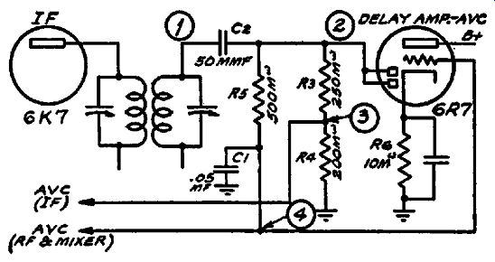
Fig. 7-22. A system of delayed avc used in the Motorola Golden Voice receiver in which the delay voltage is amplified and automatically controlled.

Some receivers employ a type of avc system in which the control voltage is both amplified and delayed. In Fig. 7-22, for instance, the circuit of the 1936 Motorola Golden Voice avc system is shown. The resistor R6, through which the plate current of the 6R7 tube flows, provides a negative bias for the diode rectifier and the control grid of the 6R7. As soon as the signal level reaches a value sufficient to overcome this bias, current flows in the diode circuit, increasing the negative bias on the 6R7 grid and consequently decreasing the plate current as well as the current through R6. Thus the delay voltage due to the voltage drop across R6 is decreased and, at high signal levels, the action is similar to that of a simple avc system. Note that RS and R4 form a voltage divider and that the i-f control voltage is taken off at the junction of these two resistors. The actual control voltage thus applied is approximately one-half that applied to the r-f and mixer stages.

Tracing the signal from point 1 to point S checks the functioning of the condenser CS. Voltage measurements at points S, 3 and 4 will localize faults in the avc distribution system just as was described before.

Quiet A VC Systems

We mentioned earlier in this section that the purpose of qavc is to prevent excessive noise when tuning between stations. In commercial broadcast receivers this is accomplished by blocking the signal passage in either the i-f, a-for detector stage until the signal strength reaches a certain predetermined value. Thus weak ...

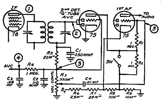
Fig. 7-23. A quiet avc circuit which is representative of those of the blocked audio type. The increased voltage developed across R2 during intervals of low input signal blocks the first a-f stage.

... signals and background noise of the same strength are not reproduced. The signal level at which this blocking takes place is termed the "squelch" level. In some circuits this squelch level is adjustable to meet the varying noise levels present in different locations; in others, a switch is provided to remove the squelch voltage so that simple avc action takes place.

Fig. 7-23 shows a representative qavc circuit of the blocked audio type. This is the circuit used in the Philco Model 810 PA receiver. You will note that the diode section of the first 75 tube is used as the second detector and also as the avc tube. The avc voltage is fed to the controlled tubes through the filter, R4-CS, while the negative voltage which is applied to the grid of the triode section of the 75 is taken directly from the high side of the volume control R3. The plate of the triode section which serves as the "Q" tube, is connected to a positive point on the voltage divider through R2. The triode section of the second 75 tube is employed as a first a-f amplifier and is controlled. The diode section of this tube is not used. Connecting the cathode to a positive point on the voltage divider enables a negative bias to be applied to the control grid of the 75 a-f tube equal to the voltage drop across RB. Noise suppression is accomplished in the following manner: when the input signal to the detector diode is high, a high negative voltage is present across R3. Since the grid of the "Q" tube is connected to this point this high negative voltage reduces the plate current through Rt to a very low value. Consequently there is practically no voltage drop across R2 and the negative bias on the first a-f grid remains at its normal value. However, when the signal input to the diode is low, the bias on the "Q" tube grid is likewise low, plate current flows through R2 and the bias on the a-f grid is increased. Since this is a high-mu tube, a small increase in the negative bias is sufficient to reduce the 6ignal amplification to zero.

Once the operation of the circuit is thoroughly understood, signal tracing procedure becomes almost self-evident. We know that the modulated i-f signal should be present at points t and 2, so we check it at these points. Since the diode load is by passed by C1 and C2, the intermediate-frequency signal should be very small at point S. However, the a-f component will be large, because C1 and C2 are too small in capacity to by-pass the a-f signal. At point 4, we can check the filtering of the a-f component.

At point 5 we can test the operation of the noise-suppression action by noting if the d-c voltage at point 5 becomes less positive as the modulated signal applied to the receiver is increased. It should be noted that the d-c bias voltage will be normally positive with respect to ground though negative with reference to the cathode because the cathode is connected to a positive voltage point on the voltage divider. It is assumed, unless otherwise stated, that the voltage measurements are being made with reference to ground. All measurements are made with the switch across R2 open-when this switch is closed R2 is shorted out, therefore the grid voltage at point 5 cannot change and noise suppression does not take place.

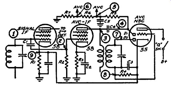
Fig. 7-24. A system of noise suppression which acts by blocking the signal i-f amplifier stage. This is done by the voltage drop across R1 due to the large plate current of the triode section during periods of low input signal.

The circuit shown in Fig. 7-24 is a partial schematic showing the noise suppression and avc system employed in the RCA Model R-78 receiver. Two i-f stages are used, one to feed the second detector and the other to amplify the signal voltage which feeds the avc rectifier. When a modulated signal is fed to the receiver input, the i-f signal at point 1 is coupled to the control grid of the avc-i-f tube at point 2. The amplified i-f signal at point 3 is fed to DJ, a diode plate of the 55 tube and the avc voltage is developed across the network composed of R5, R6 and R7, as points 5 and 6.

The noise-suppression circuit is composed of the diode D2 and the triode section of the 55 tube. The amplified i-f signal at point 3 is coupled to Di by means of the i-f transformer. This signal is checked at point 7. The resulting negative voltage across the diode load R4 serves to bias the grid of the 55 tube. Since the cathode of the 55 returns to ground through the cathode resistor of the first i-f tube, any increase in cathode current in the 55 tube will cause an increase in the control-grid bias of the first i-f tube. When the signal level at point 7 is low, the negative bias on the grid of the 55 tube is low and the plate current is high.

Therefore, for weak signals the cathode voltage at point 9 is greatly increased; thus the amplification of the i-f tube is reduced and the signal applied to the second detector becomes very low.

On strong signals the cathode voltage at point 9 is low and the gain of the first i-f tube depends only upon the regular avc action.

In checking this circuit by signal tracing, we need only follow the normal course of the signal to points 4 and 7 and then check the resulting d-c potentials which form the control voltages at points 5, 6, 8 and 9. These tests should be made with the plate circuit switch of the 55 closed, since noise-suppression action can not otherwise take place.

There are a great many other noise-suppression, or qavc circuits, some of which operate on the second detector tube, but all function fundamentally in the manner of the two described above.

The analysis of these circuits, as well as those of the simpler avc circuits previously described, should enable the more difficult problems which arise in the servicing of such circuits to be solved more easily.

It should not be assumed that all the operations described in the testing of each of these circuits should perforce be followed in every servicing job which involves these circuits. The simplest and quickest tests which give the information required, based on the symptoms or the customer's complaint, are usually all that is necessary. Most of these simple preliminary tests can be made by giving the receiver an operating test on a standard broadcast signal.

Suppose, for instance, that the customer complains that in tuning from one station to another, the signal temporarily disappears, then gradually builds up to normal volume. This may be caused by a change in the time constant of the avc filter network. We can check the time constant by tuning quickly from a strong station to a weak station and noting if too much lag is evident in the operation of the ave. If such is the case, then our tests must be applied directly to the avc filter circuit or the individual grid filters, first checking the components to make sure they are of the value specified by the manufacturer. The reason for this check is that the receiver may have been serviced and a condenser or resistor of the wrong value may have been substituted for the one originally installed.

A quick check of avc operation can be made by simply placing the voltmeter probe upon the control grid of one of the controlled tubes, and noting the change in voltage which should take place in tuning from a strong broadcast signal to a weaker one.

Signal tracing in avc circuits can be done with an oscillator and output meter. In such cases, the output meter should be placed at a point such as point 4 in Fig. 7-23, and the signal voltage should be applied to points ahead of the filter circuit. For instance, by feeding a strong audio signal at point 3 and measuring the audio output at points 3 and 4, the effectiveness of the filter in reducing the audio signal can be determined. The output meter for such work should be of the vacuum-tube type, of high input impedance, since its input capacitance is in parallel with the circuit to which it is connected. In using the test oscillator for diode circuit testing, the modulated signal preferably should be fed through a blocking condenser to the primary of the last i-f transformer. If connected directly across the diode, the test oscillator attenuator will short-circuit the diode lead and mis leading results will be obtained.

SIGNAL TRACING IN AUTOMATIC FREQUENCY CONTROL CIRCUITS

Modern broadcast receivers, particularly those which employ broad-band i-f transformers, are often mistuned by inexperienced owners. When the desired station may be heard over a wide range of adjustment of the tuning dial, as is often the case with sensitive sets having automatic volume control, it may be difficult to determine the precise point of resonance. Yet, if the receiver is not precisely tuned, distortion results and the performance of the receiver suffers. Inaccuracies in tuning also result from oscillator drift and mechanical difficulties in electric and other automatic tuning systems. Automatic frequency control is a means for correcting such errors in tuning. This correction is accomplished automatically by special circuits designed to shift the frequency of the superheterodyne oscillator so that the proper i-f signal results even when the oscillator is mistuned nearly 10 khz.

Automatic frequency control operates upon the oscillator of the superheterodyne receiver because the tuning of this circuit is far more critical than that of the r-f or mixer sections. When this circuit is tuned approximately to the correct frequency, automatic frequency control (abbreviated afc) serves to raise or lower the oscillator frequency until the correct intermediate frequency results.

To understand how afc functions, let us first consider the properties of an inductance. We know that if a given inductance has a certain impedance at one frequency, it will have a higher impedance to a slightly higher frequency and a lower impedance to a slightly lower frequency. Now, if we can make a vacuum tube vary in impedance with frequency in the same manner as an inductance, the vacuum tube can be used in a circuit in place of a variable inductance. This is accomplished in afc circuits by varying the grid bias on a tube which is arranged to act as an apparent inductance which varies automatically in accordance with changes in frequency above or below the desired point so that the tube impedance varies with frequency.

The tube which is thus transformed into an apparent inductance is called the oscillator control tube and the tube which causes the oscillator control tube to perform in this manner is termed the discriminator. The proper functioning of any afc circuit is based upon proper performance of these circuits, so let us see how they operate.

A typical discriminator circuit is shown in Fig. 7-25. The inductance Lt is tuned by C P to the intermediate frequency used in the receiver and is inductively coupled to the secondary coils L2 and L3. The secondary is likewise tuned to resonance with the intermediate frequency. When an i-f signal is present, this signal voltage causes a rectified d-c voltage in the secondary circuit to be developed across RJ and R2. The signal voltages applied to the two diodes are equal and opposite because the secondary of the discriminator transformer is center-tapped.

Since R1 and R2 are likewise equal, the resulting d-c voltages across R1 and R2 are equal.

A portion of this i-f signal voltage is also fed to the secondary of the discriminator transformer through the condenser, C, and the phase relations of this signal voltage E1, with respect to EfJ and ES change with frequency so that the control voltage, at …

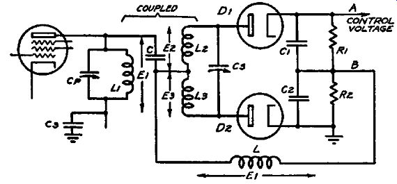
FIG. 7-25. A basic discriminator circuit used in afc systems to provide the voltage required for controlling the oscillator frequency.

… point A, changes in a positive or negative direction as the i-f signal varies above or below the proper frequency. This control voltage is applied to the control grid of the oscillator control tube, causing its impedance to vary in accordance with the changes in the applied control voltage. Since the oscillator control circuit is shunted across the local oscillator in the receiver, these changes in impedance serve to vary the oscillator frequency. When properly adjusted, the afc circuit will compensate for errors in the oscillator frequency due to mistuning by automatically changing the oscillator frequency to the value required to produce the desired intermediate frequency.

Fig. 7-26 shows the oscillator control tube and oscillator circuit of a typical afc system. The afc control voltage is applied to the oscillator control tube grid through the filter network R5-C5 and R4-C4, which performs the same functions as similar filters in avc systems. The network R3-C4 is used to apply the oscillator signal to the oscillator control tube so that it draws a lagging current from the oscillator tuned circuit. The magnitude of this lagging current is controlled by the afc bias voltage applied to the control grid. When the bias voltage changes in a positive direction, the plate current of the oscillator control tube is increased and its apparent inductance is decreased. When the bias voltage becomes more negative, the plate current is decreased and its apparent inductance is increased. Thus the oscillator control tube acts as a variable inductance shunted across the oscillator tuned circuit.

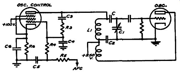
FIG. 7-26. A basic oscillator control circuit showing the connections to the oscillator circuit.

Since this apparent variable inductance is shunted across the oscillator coil, it acts to reduce the effective inductance of the circuit. When the inductance in any circuit is lowered, its resonant frequency is raised, and when the inductance is in creased, the frequency is lowered. When all circuits are properly adjusted, the local oscillator should produce the proper beat with the r-f signal to give the desired intermediate frequency. Then, should the oscillator deviate from this frequency, the resulting intermediate frequency will change by the same amount. This brings the afc control voltage into action, changing the bias on the oscillator control tube grid in either a negative or positive direction, as required to increase or decrease the effective inductance of the circuit and thereby restore the proper oscillator frequency.

A complete discussion of the manner in which this is accomplished is given in the book "Automatic Frequency Control Systems" by John F. Rider.

We have seen that the operation of afc circuits has much in common with that of avc circuits. In superheterodyne receivers, the i-f signal serves to operate each type of circuit. In each, the i-f signal is applied to a rectifier and the resulting d-c voltage is used to control another circuit. In avc circuits, the gain of con- trolled tubes is governed; in afc circuits, the oscillator frequency is controlled. Often these two functions are combined in a standard afc circuit. Now let us apply signal tracing to a typical circuit as employed in a commercial broadcast receiver.

The afc circuit used in the General Electric Model E-101 receiver is shown in Fig. 7-27. As you will note, both afc and avc action is obtained with this circuit. A simple preliminary test ...

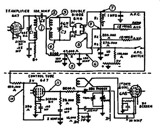
FIG. 7-27. The afc circuit used in General Electric 1937 12- and 15-tube receivers.

... should first be applied to determine the need for servicing of this circuit. This is done by connecting the receiver to a good antenna and tuning in a strong local broadcast station with the afc switch closed, which renders the afc system inoperative. Then open the afc switch and note if there is any change in the character of the signal as reproduced by the speaker. If the signal is still free from distortion, the afc circuit is either functioning normally or is totally inoperative. Now, with the afc in operation, detune the receiver slightly and note if the signal remains clear. If it does, then again close the afc switch and listen for a change in the signal clarity. Some distortion should be evident because the afc circuit is now inoperative. The purpose of this test is to find out if the afc is correcting for detuning by compensating for the change in oscillator frequency.

Signal tracing is done by first checking the signal frequency at point 1. This frequency should conform to the intermediate frequency specified by the manufacturer. These tests are made with a tuned vacuum-tube voltmeter. Then move the v-t voltmeter probe to point 2. Presence of a strong signal at this point indicates that the coupling condenser C2 is functioning properly. The i-f signal likewise should be present at points S and 4, and when the discriminator transformer is properly center-tapped, these signal voltages should be equal. The signal should be very weak at point 5, since the r-f choke and by-pass condenser form a filter circuit, and should be still further attenuated at point 6, due to the action of the resistance-capacity filter. Points 7 and 8 are by-passed both for intermediate and audio frequencies, so no signal voltages should be present at any of these points. At points 10 and 11, the oscillator frequency, representing the sum of the intermediate and r-f signal frequencies, should be present. Note that the control grid of the oscillator control tube is by-passed with only a 5-µµf condenser; therefore the test probe and its cable should be so designed that very little capacitive load is placed on this circuit or the oscillator signal will be by-passed when the tuned v-t voltmeter is connected. This effect is likewise an important consideration in the testing and adjustment of any tuned circuit, since even the slightest capacity so introduced will serve to detune the circuit to some extent. Any conditions observed during the progress of this signal tracing procedure which are not in accordance with the normal results specified above call for investigation of the components involved at the point where the trouble is first noted.

As has been pointed out before, the rectified d-c voltages across the cathodes of the discriminator 6H6 are normally equal and of opposite polarity. This means that the d-c voltage from point 9 to point 8 should equal that from point 9 to point 7 when the discriminator transformer secondary is accurately tuned to the intermediate frequency. Since these voltages are of opposite polarity with respect to point 9, the voltage at resonance between points 7 and 8 should be zero. Point 7 will become either positive or negative with respect to point 8 as the intermediate frequency increases or decreases. This varying voltage is applied to the control grid of the 6J7 control tube at point 10.

In checking these voltages, it is assumed that one terminal of the voltmeter is connected to ground. Since both points 8 and 7 return to a point on the voltage divider which is 3 volts negative with respect to ground, the normal voltage reading at each of these points is -3 volts. This negative voltage forms the fixed control grid bias for the oscillator control tube.

In aligning the afc circuit by means of voltage measurements, the first step is to align the r-f, oscillator and i-f stages in the conventional manner with the afc rendered inoperative by closing the afc switch. Then, with a strong signal applied to the receiver input terminals, the set should be tuned to resonance and the afc switch opened. With the voltmeter probe connected to point 7 and ground, the voltage reading should be noted. Since the preliminary test on a broadcast signal would indicate the need for alignment, the voltage reading at point 7 will be greater or less than -3 volts. Whatever reading is secured, adjust C1 until it is a maximum. The primary of the discriminator transformer is then properly aligned.

The secondary circuit is then aligned by simply adjusting C3 until the voltage reading at point 7 is -3 volts. Then, when the afc switch is opened and closed the voltage reading should not change. If it does, then the fixed bias voltage is not -3 volts and the voltage divider should therefore be checked. In any event, the discriminator secondary tuned circuit is properly adjusted when the voltage reading from point 8 to ground is the same as that from point 7 to ground.

The afc circuit is shown in Fig. 7-28 is employed in the Midwest Model 18-37 receiver. The discriminator circuit is somewhat simpler than the one just described, the filter network being omitted. The control-grid bias for the oscillator control tube is obtained by biasing its cathode rather than by using a fixed volt age in series with the afc voltage. A resistance-capacity filter in the plate circuit of the oscillator control tube serves to isolate the power supply from the oscillator control circuit and to provide hum filtration for the oscillator control tube plate.

Signal tracing and alignment proceed along the same lines as for the previously described circuit. Since one cathode of the 6H6 discriminator is at ground potential, the discriminator secondary circuit will be precisely aligned when the voltage reading from point 5 to ground is zero. With a strong signal being received, opening and closing the afc switch should cause no change in the zero voltage reading from point 5 to ground. With the afc in operation, detuning the receiver slightly above or below the proper tuning point should cause a corresponding change in the d-c voltage reading at points 5 and 6. The readings at each of these points should be the same.

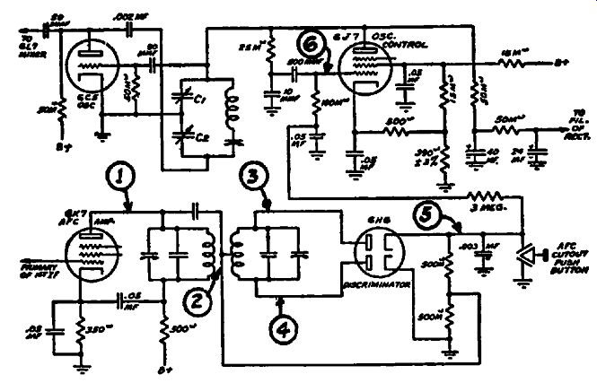
Fig. 7-28. The afc circuit used in the Midwest Model 18-37 receiver.

A separate i-f stage is used to feed the signal to the discriminator circuit.

Hum may be introduced in the receiver due to insufficient filtration of the afc system. Often this may be quite simply checked by removing the oscillator control tube, retuning the receiver, and noting if the hum disappears. If it does, then of course the trouble is localized to that section of the circuit. This also may be checked by signal tracing, noting the hum level in the oscillator plate circuit as described in the section on signal tracing in oscillator circuits. This hum modulates the oscillator and there fore the resulting i-f signal which is amplified before detection.

Thus even a very low hum level in any circuit which connects to the oscillator may be amplified sufficiently to prove annoying.

The most successful results, with any system of testing, are obtained when the operation of the circuits involved is thoroughly understood. Therefore particular attention should be devoted to the study of the circuit itself rather than to following blindly the test routine prescribed. In this manner, short cuts will suggest themselves, time will be saved and more work will be turned out with less effort. To enable you to do just this is the purpose of this book.

AUTOMATIC VOLUME EXPANSION

During the broadcasting of a program at the studio, the audio output which modulates the transmitter is constantly monitored by the control man so as to insure the greatest efficiency in operation and the widest station coverage. In some transmitters, too, this monitoring is done automatically by a system known as volume compression. During periods when the average sound level of the music being broadcast is high, the gain of the modulation amplifier must be reduced to prevent overmodulation of the carrier. On the other hand, when the average audio level is low, the gain of the amplifier must be raised so that the level of the music will be greater than the noise and hum level of the carrier. Thus the overall volume range of the transmitted program is com pressed within a limited range so that the program as received in the home is not precisely of the same range as that heard in listening to the broadcasting orchestra in the studio.

Volume expansion circuits compensate for this reduction in volume range at the transmitter by automatically raising the volume in accordance with the average audio level. An ideal type of volume expander would be one in which the degree of volume expansion exactly compensated for the amount of compression at the studio so that the resulting audio output of the receiver is exactly the same as the signal reaching the studio microphone. This cannot be attained, since the degree of monitoring varies in different studios and often on different programs in the same studio. However, volume expansion is very satisfactory in the reproduction of records, since the amount of volume compression during recording does not vary so greatly.

There are various ways of securing volume expansion, but nearly all are based on some method of varying the gain of an audio amplifier tube so that the stage gain is increased as the signal strength increases and decreased as the signal strength decreases. One exception is a method which uses a network of linear and non-linear resistances in the form of a bridge, which is shunted across the voice coil and output transformer secondary.

This bridge is so arranged that the output power delivered to the voice coil increases with an increase in applied signal to a greater degree than would occur if the network were not used. By the same action, weak signals are made weaker than they otherwise would be.

A fundamental circuit showing the first-mentioned type of volume expander, which is most widely used, is shown in Fig. 7-29. This one is described in an application note issued by the RCA Manufacturing Company, Inc. The 617 acts as an audio ...

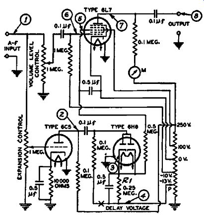
Fig. 7-29. An automatic volume expansion circuit. The gain of the 6L7 is automatically controlled in accordance with the average volume level.

... amplifier and its amplification is controlled by the expander section, consisting of the 6C5 amplifier and 6H6 rectifier. In operation, when the expansion control is at minimum setting, the 617 functions as an ordinary audio amplifier. When the expansion control is advanced, a portion of the audio signal voltage which is fed to the 617 is likewise fed to the 6C5. This signal voltage is amplified by the 6C5 and applied to the 6H6 rectifier. As a result of rectification, a d-c voltage is developed across RI of positive polarity with respect to ground. This positive voltage is applied to GS of the 6L7 and serves to reduce the normal negative bias voltage for this grid. As this grid voltage becomes less negative, the mutual conductance of the 6L7 is increased, thus increasing its gain. Since this increase in gain is greater as the signal voltage applied to the 6H6 is increased, the result is that strong signals are amplified more than weak ones. In effect, this means that during reception of music, if one note normally were received at twice the audio signal level of another, more than twice the audio signal level would appear at the output terminals of the volume expander. The amount by which the differences in level between two signals is amplified depends upon the position of the expansion control. Maximum expansion occurs when the expansion control is at maximum setting, since then the widest variations in signal and control voltages result. The signal level at which volume expansion starts to operate may be delayed by inserting a negative voltage in series with the diode return at the point marked (x) in the diagram.

For a preliminary operating test, an audio signal should be fed to the a-f input terminals of the expander. If the expander circuit is a portion of a radio receiver, a modulated r-f signal may be applied to the receiver input terminals. The audio component, after detection, will then serve to actuate the volume expansion circuit. With the expansion control at minimum setting, advance the volume control until the signal as reproduced by the speaker is of moderate volume. Then advance the expansion control.

The sound volume should increase, providing the applied signal voltage is high enough to overcome the delay voltage, if any, used in the expansion circuit. A signal level at point 1 of the order of 1 volt should be adequate for most test purposes. If no increase in volume results from this test, the circuit should be checked.

In signal tracing, the audio signal should first be checked at point 1. Then, with the expander control advanced to maximum setting, check the signal at point 2. The signal voltage should be several times greater at this point-the actual gain will depend upon the design of the particular circuit employed. At point 3, no audio signal should be present, but the d-c voltage drop across R1 from rectification in the diode circuit should create a voltage which is positive with respect to point 4, This represents the control voltage applied to the 6L7 and can be cheeked directly at point 5 on the diagram. The change in this control voltage should cause a corresponding change in the signal level at point 7.

The audio signal therefore should be checked at point 7 and also at point 8 to check the blocking condenser. The location of faults by this method of testing follows along the same lines as was previously described for other control circuits.

An example of the use of another type of volume expansion in a radio receiver is shown in Fig. 7-30. Basically the method of operation will be clear from the small insert diagram. A 100,000 ohm resistor in series with the plate resistance of the 6K7G expander tube forms a voltage divider across the input to the power amplifier stage. As a result of this connection, the grid of the output stage receives only the voltage which is developed across the plate resistance of the 6k7G, represented in the small dia gram (a) by a resistor within a circle. Automatic expansion of volume is achieved in this circuit by automatically varying the value of the plate resistance in accordance with the average audio or modulation level. During periods when the modulation level is high, the bias on this tube is likewise high, and consequently the plate resistance of the 6K7G also is high. The average volume level is therefore increased because of the voltage-divider action, of which the plate resistance of the 6K7G tube forms the lower portion.

On the other hand, when the modulation percentage is low, the bias on the 6K7G tube is likewise low, its plate resistance is decreased and the fraction of the total audio voltage which reaches the grid of the output stage is likewise small. In this way, an automatic expansion of the volume is secured.

Let us now examine the function of the several circuit components in somewhat more detail. Referring again to Fig. 7-30, the audio voltage produced across the volume control in the full wave diode-detector load circuit is amplified by the triode section of the 6Q7G, and the output of this stage is fed to the grid of the 6N6G output tube through a resistor-condenser network. Automatic biasing of the 6K7G, in accordance with the average output level, is accomplished by feeding the audio voltage across the output of the 1st a-f stage through a .006-µ.f condenser and a 1-meg resistor to the grid of the 6.J7G expander-amplifier. This tube acts as a rectifier-amplifier and produces a pulsating d-c voltage across the 470,000-ohm resistor in its plate circuit. This rectified d-c voltage is filtered by the 1-megohm resistor and 0.2 and 0.3-p.f condensers before being applied to the suppressor grid of the 6K7G expander.

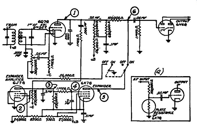
FIG. 7-30. An automatic volume expansion circuit. The plate resistance of the 6K7G is varied automatically to control the input signal to the 6N6G output stage.

As the signal level applied to the 6J7G increases, the rectified voltage across the plate resistor of the tube increases, thereby increasing the negative d-c bias on the suppressor grid of the 6K7G. This increasing suppressor grid bias causes the plate resistance of the 6K7G expander tube to increase correspondingly as the percentage modulation of the broadcast signal increases and the final audio voltage reaching the output tube grid increases beyond the value it otherwise would have without expansion.

The double-pole double-throw switch makes operation of the expansion circuit optional. When the volume expansion switch is in "off" position, a 56,000-ohm resistor is shunted across the tapped section of the volume control and the plate of the ex pander tube is disconnected from its coupling to the input circuit of the output tube. This serves to equalize the volume level with the switch in either position.

Assuming that the signal has been traced through the rectifier circuit, we may check the audio gain at point 1. A test at point 2 which indicates the presence of the signal at this point is evidence of proper coupling between points 1 and 2. The a-f signal should be weak at point S, due to filtration by the .3-µ.f condenser, but the d-c voltage resulting from rectification may be checked at this point and point 4, Increasing the receiver input signal level or the percentage modulation should cause a corresponding decrease in d-c voltage at point 4. The a-f signal will appear at point 5.

Doubling the input signal voltage should cause far more than double the signal voltage at point 5. Proper functioning of the switch connection may be determined by tracing the signal from point 5 to point 6. The signal levels, with volume expansion operating, should be the same at these two points.

Automatic Bass Amplifier

In receiving musical broadcast programs at low volume levels, it is a characteristic of the human ear that the low notes seem to be reproduced at lower volume than the high notes. Yet, when the overall volume level is raised, the proper proportionate strength is established. Automatic bass control is a means of automatically providing increased bass response at low volume levels to correct for this psychological condition, and proportionately less increase as the overall volume level is increased. In addition, a manual adjustment is provided which enables the listener to vary the amount of bass amplification in accordance with his own preferences. The latter adjustment then becomes in effect a bass tone control, although the manner of operation is essentially different from the conventional tone control.

The manner in which the automatic bass control action functions is evident when the simplified diagram of Fig. 7-31 is analyzed. A portion of the output of the 6F6G driver stage is coupled to the diode plates of the 6R7G and this audio signal is rectified. The resulting d-c voltage across the 500,000-ohm diode load is filtered through the 1.0-megohm resistor and .45-µ.f condenser and fed over to the 6K7G bass amplifier tube. In this way the d-c bias on the 6K7G is made to vary in accordance with the strength of the signal at the output of the driver stage-in other words, in accordance with the output level of the receiver. When the output level is low, the bias voltage on the 6K7G likewise will be low, and the gain of the bass amplifier will be greatest; on the other hand, when the output level is high, the bias will be high; therefore the gain of the 6K7G will be reduced and the amplification of the bass channel will be accordingly lower. A ...

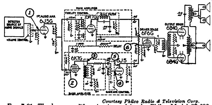
Philco Radio / Television Corp.

Fig. 7-31. The bass amplifier circuit used in the Philco Model 37-690. The gain of the bass channel is controlled automatically in accordance with the average volume level.

...delay action is incorporated in the automatic bass control circuit by applying a negative bias voltage on the diode load resistor return. For this reason, the diode will not begin to rectify and thus furnish a voltage to control the gain of the bass amplifier until the output level of the receiver reaches a certain value.

In signal tracing, since we are primarily concerned with the amplification of low notes, the audio signal preferably should be in the neighborhood of 100 cycles. The signal may be either a modulated radio frequency, applied to the input terminals of the receiver, or an audio signal applied to the first a-f grid at point 1.

If no such low-frequency source is at hand, a broadcast signal of orchestral music or a phonograph record with low notes in the selection may be used for test purposes. For signal sources which are of constant audio frequency, signal voltage measurements may be made.

A signal check should be made at point 2 and the signal level of the main amplifier raised by adjusting the volume control until a d-c measurement at point 2 shows a slight increase in the negative bias voltage. Then check the audio signal at point 3. The signal strength should be a maximum at this point. Now again advance the volume control setting of the main amplifier. This should cause an increase in the negative d-c bias voltage at point 2 and a corresponding decrease in gain of the a-f signal at point 3.

Now place the test probe at point 4 and advance the bass amplifier control to maximum setting. Low-frequency notes in broadcast program reception should appear more pronounced than the higher ones at this point because of the high-frequency filtering action of the series resistor Rt and shunt condenser, Ct, employed in the coupling to the grid of the 6J5. At point 8, the signal from the main amplifier combines with that of the bass amplifier and a portion of the main amplifier signal voltage also will be present at point 5. To isolate the bass amplifier signal, the plate load resistor of the 6R7G may be open-circuited, thus preventing any signal voltage from the main amplifier from reaching point 6. The output of the bass amplifier may then be checked independently at either point 5 or point 8.

SIGNAL TRACING IN INVERSE FEEDBACK CIRCUITS

Inverse feedback, which is also known as negative feedback or degeneration, is a method of improving the performance of an amplifier by feeding back a portion of the output signal voltage to an input circuit in such manner that the feedback voltage opposes the phase of incoming signal. As a consequence, the frequency response is made more uniform, the stability is increased and harmonic and phase distortion are reduced. In output circuits, inverse feedback produces a desirable damping action on the speaker when high plate-impedance output tubes are used.

This damping action is similar to that which would result if the best triodes were used and enables the speaker voice coil to repro duce rapidly changing frequencies more faithfully. This improved performance is obtained at a sacrifice of amplifier gain, so additional gain is often incorporated in such amplifier designs when needed.

Inverse feedback is the opposite of regeneration, hence the name "degeneration". In regeneration, the feedback voltage aids the input signal voltage and consequently the overall gain of a tube and circuit is increased. In degeneration, the feedback signal bucks the incoming signal so stage gain is decreased. Since the feedback signal becomes stronger, and therefore the bucking action becomes greater, as the stage gain increases, inverse feed back tends to equalize the gain over the frequency range of the amplifier. This effect is often further increased by designing the inverse feedback network so that the feedback voltage is greater in proportion to the increase in amplifier gain at certain frequencies so that maximum compensation for non-uniform frequency response is secured with minimum loss in amplification. Since the feedback voltage contains any hum or distortion which may originate at the point where it is derived, such faults are also bucked out by this method. The measure of improvement depends upon the amount of feedback which is introduced; complete compensation cannot be secured since there must always be some fault in the signal before the feedback system can operate to correct it. But a considerable improvement in fidelity results over that which is normally secured with the same components without inverse feedback.

FIG. 7-32. An inverse feedback circuit in which the feedback signal is fed from the output circuit to the cathode of the second audio stage.

You will find in Fig. 7-32, the inverse feedback circuit used in the G.E. type E-155 receiver. The path of the feedback voltage is indicated by the heavy lines. The audio signal voltage, which appears across the secondary of the output transformer, is fed back to the cathode circuit of the 6F6 driver tube through a 180-ohm resistor and 2-µ.f condenser and is impressed across a 50-ohm resistor in series with the 1000-ohm cathode biasing resistor. At high frequencies, the reactance of the 2-µ.f coupling condenser is low so that the feedback voltage introduced in the cathode circuit is high, amounting to approximately 20 percent of the audio voltage present at the output transformer secondary.

At low frequencies the reactance of the coupling condenser is high so that the feedback voltage developed across the 50-ohm resistor becomes small. Since the gain of the amplifier is reduced as the feedback voltage is increased, we see that at higher frequencies where the amplifier gain is normally high, the feedback voltage tends to reduce the gain considerably while at low frequencies, where the amplifier gain normally decreases, the decrease in feed back voltage causes only a small reduction in overall gain. Thus a degree of additional compensation is introduced which increases the normal improvement in frequency response which results from inverse feedback.

In signal tracing, the feedback signal voltage cannot easily be checked independently of the incoming signal when both are present simultaneously in all circuits because they differ only in phase and magnitude. We should require special equipment to check the phase of these voltages. The simplest method of testing this inverse feedback circuit is to check its operation by noting its effect on the gain of the amplifier. If we open the inverse feedback network at either points 1 or 2 in Fig. 7-32, the amplifier will function without inverse feedback. Under such conditions, the overall gain should be increased. By applying an audio signal to the 6C5 grid, or by feeding a modulated r-f signal to the receiver input circuit, and noting the output voltage across the voice coil with and without the inverse feedback network in operation, it is possible to tell if the circuit is in operating condition.

A more accurate test may be made by opening the inverse feed back network at point 1 and connecting the lead to the 180-ohm resistor to a variable-frequency audio oscillator. By checking the audio voltage at point 3, with the oscillator voltage maintained constant, the frequency characteristic of the feedback net- work may be determined. In this circuit, the audio voltage from point 3 to ground should be approximately 3 percent of that applied at point 1 when the frequency fed to the network is 50 cycles and should increase to approximately 20 percent as the frequency is increased to 5000 cycles. Since this is merely a test of the frequency characteristic of the network, the amplifier need not be in operation while this test is made.

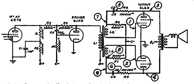
FIG. 7-33. Inverse feedback is used in both the driver and output stages as shown by the heavy-line circuits.

In Fig. 7-33 the audio amplifier section of the Philco Model 38-116 receiver is shown. In this circuit negative feedback is employed both in the driver and push-pull output stage. In the driver stage, the signal voltage at the plate of the 6J5G is fed back to the grid of the same tube through the network shown in the heavy lines. R3 is used to limit the loading effect of the parallel network consisting of the plate resistance of the 6R7G tube and its load resistor, R1. The combined effect of this load across the input circuit of the driver reduces the inverse feedback voltage to approximately 8 percent. The reduction in gain resulting from this feedback voltage may be checked by comparing the output signal voltage at the plate of the 6J5G plate, with the 500,000-ohm resistor disconnected-thereby rendering the feed back circuit inoperative-with that secured when the 500,000-ohm resistor is in the circuit.

Inverse feedback in the output stage is accomplished by means of the voltage divider network composed of RB, CS and R6, for one tube and R9, C4 and R7 for the other tube. When the in verse feedback circuits are performing normally, the signal volt ages at points 5 and 8 are equal; likewise at points 7 and 8.

Inequalities of the signal voltages at points 1 and 2 and at points 3 and 4 will affect the equality of the feedback voltages at the points mentioned, even though the components are functioning properly. The effect of inverse feedback on the gain of each out put tube can be checked in the same manner as was described for the driver stage. This test may be made by opening the feed back network at either point 3, 5 or 7 for the upper network and either point 4, 6 or 8 for the lower network.

Effect of Inverse Feedback on Amplifier Gain

We have mentioned that inverse feedback reduces the gain of an amplifier in which it is used. This reduction in gain is considerable; if 10 percent of the output voltage is fed back by this method to an input stage, the overall gain of the amplifier is reduced to about 9. It makes but little difference what the gain of the amplifier would be without negative feedback. For in stance, if the gain were 100 without negative feedback, the gain with 10 percent negative feedback would be 9.1. And, if the normal gain were 200, with 10 percent negative feedback the overall gain would be reduced to 9.5. With greater percentages of negative feedback, the uniformity is even more pronounced.

For 20 percent negative feedback, the gain of an amplifier which would be 100 without feedback is reduced to 4.8; yet, if the nor mal gain were 200, with the same amount of feedback the gain would be reduced to 4.9. With this in mind, then, we can show a graph which gives the approximate amount of gain we should expect in any amplifier in which negative feedback is used and where the normal gain is 100 or more. These gains shown in Fig. 7-34 are figured on the assumption that the normal gain of the amplifier without feedback is 100. When the gain of the stages included in the feedback circuit is greater than 100, the values shown in the figure will still be approximately correct.

However, for gains less than 100, and especially for low percent ages of feedback, the overall gain will be smaller than that shown by the curve.

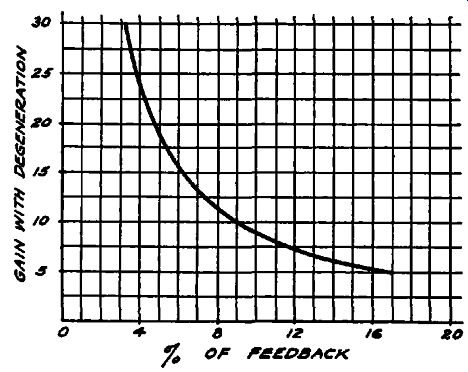
Fig. 7-34. The gain of an amplifier with degeneration de creases as the percentage of feedback increases. This curve is on the basis of a gain of 100 with no feedback.

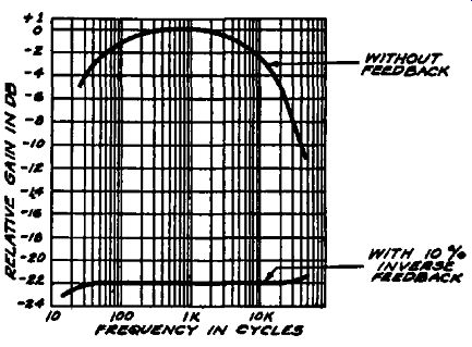
Fig. 7-35. Response o an amplifier with and without inverse feed back. Note the improved frequency response effected by the use of feedback.

The curve given in Fig. 7-34 will serve to make possible a quick check of the gain in any amplifier employing negative feedback and thereby to determine the need for servicing. It is obvious, if the negative feedback circuit were inoperative, that the gain in the amplifier would be greatly increased.

The action of negative feedback in correcting frequency distortion is shown graphically in Fig. 7-35. The feedback used was about 10 percent. Note that, without feedback, the amplifier response is down 10 db at 30 khz and 4 db at 30 cycles while with feedback, the response is flat to within ½ db over the same range.

The overall gain, of course, is greatly reduced-approximately 22 db below that obtained without feedback.

When inverse feedback is applied to an output stage only, as is illustrated in the push-pull 6L6 stage shown in Fig. 7-33, the reduction in gain is not so pronounced. If the normal stage gain is 15, 10 percent negative feedback will reduce the gain to 6. If the normal gain is 10, the same amount of inverse feedback will reduce the gain to 5. These figures will serve to give an idea of the gain which may be expected in typical amplifiers employing negative feedback.