AMAZON multi-meters discounts AMAZON oscilloscope discounts
A capacitor is one of the most common components used in electronics, but is probably one of the least understood. As in the case of inductors, a capacitor is a storage device. An inductor stores electrical energy in the form of an electromagnetic field, which collapses or expands to try to maintain a constant current flow through the coil. In comparison, a capacitor stores an electrostatic charge, which increases or decreases to try to maintain a constant voltage across the capacitor.
Capacitor Types and Construction
A capacitor consists of two conductive plates with an insulator placed between them called the dielectric. The size of the plates, the thickness of the dielectric, and its dielectric constant all combine to determine the capacity, or energy storage capability, of the capacitor. The capacity can be increased through the use of larger conductive plates, thinner dielectric material, or a dielectric material with a higher dielectric constant.
Thinner dielectric yields higher capacity, but it also lowers the maximum voltage rating. Because it is impractical to manufacture (or to try to use) extremely large metal plates, capacitors are usually manufactured by rolling the foil plates (with the plastic dielectric sheets interleaved between them) into a round tubular form. Alternatively, layers of foil plates can be stacked and sandwiched, as when shuffling a deck of cards, with the dielectric sheets (usually mica, ceramic, or plastic) interleaved between them.
Basically, all capacitors can be divided into two categories: polarized and nonpolarized. If a capacitor is polarized (a step in the manufacturing process), the correct voltage polarity must be maintained when using it. A polarized capacitor will indicate which lead is to be connected to a positive polarity, and/or which lead is to be connected to a negative polarity, by means of labels or symbols imprinted on its body. Accidental reversal of the indicated polarity will destroy a polarized capacitor, and it could cause it to explode. Nonpolarized capacitors do not require any observance of voltage polarity.
The vast majority of capacitors use conductive metal foil as the plate material. The only exceptions are adjustable capacitors and trimmers.
The big difference in capacitor types is based on the dielectric material used. The two important properties of dielectric materials are called dielectric strength and dielectric constant. The dielectric strength defines the insulating quality of the material, and is a key factor in determining the capacitor's voltage rating. Dielectric constant will be explained a little later in this section.
Paper and mica were the standard dielectric materials for many years. Mica is used in special applications, and paper is still used quite often for general-purpose use. The paper is impregnated with a wax, or a special oil, to reduce air pockets and moisture absorption.
Plastic films of polycarbonate, polystyrene, polypropylene, and poly-sulfone are used in many of the newer large-capacity, small-size capacitors. Each film has its own special characteristic, and is chosen to be used for various applications according to its unique property.
Ceramic is the most versatile of all the dielectric materials because many variations of capacity can be created by altering it. Special capacitors (that increase in value, stay the same, or decrease value with temperature changes) can be made using ceramics. If a ceramic disk capacitor is marked with a letter "P" (positive change), such as "P100," then the value of the capacitor will increase 100 parts per million per degree centigrade increase in temperature. If the capacitor is marked "NPO" (neg/pos/zero) or "COG" (change zero), then the value of capacity will remain relatively constant with an increase or decrease in temperature.
If it is marked with an "N" (negative), such as "N1500," it will decrease in capacity as the temperature increases.
The term defining the manner in which a component is affected by changes in temperature is called the temperature coefficient. If a component has a negative temperature coefficient, its value decreases as the temperature increases, and vice versa. If it has a positive temperature coefficient, its value increases as the temperature increases, and vice versa. A capacitor's temperature coefficient is critical for circuits in which minor changes of capacitance can adversely affect the circuit operation. One reason why ceramic capacitors are the most commonly used type is the versatility of their different temperature coefficients. The other main reason for their widespread use is cost; they are very inexpensive to manufacture.
A ceramic capacitor marked "GMV" means that the marked value on the capacitor is the "guaranteed minimum value" of capacitance at room temperature. The actual value of the capacitor can be much higher. This type of capacitor is used for applications in which the actual value of capacitance is not critical.
Aluminum electrolytic capacitors are very popular because they provide a large value of capacitance in a small space. Electrolytic capacitors are polarized and the correct polarity must always be observed when using or replacing these devices. For special-purpose applications (such as crossover networks in audio speaker systems and electric motors), nonpolarized electrolytics are available, which will operate in an AC environment.
The aluminum electrolytic capacitor is constructed with pure aluminum foil wound with a paper soaked in a liquid electrolyte. When a voltage is applied during the manufacturing stage, a thin layer of aluminum oxide film forms on the pure aluminum. This oxide film becomes the dielectric because it is a good insulator. As long as the electrolyte remains liquid, the capacitor is good, or it can be "re-formed" by applying a DC voltage to it for a period of time (while observing the correct polarity).
If the electrolyte dries out, the leakage increases and the capacitor loses capacity. This undesirable condition is called dielectric absorption.
Dielectric absorption can happen to aluminum electrolytics even in storage. Sometimes, if an electrolytic capacitor has been sitting on the shelf (in storage) for a long period of time, it may need to be reformed to build up the oxidation layer. This can be easily accomplished by connecting it to a DC power supply for approximately an hour. Remember to observe the correct polarity, and do not exceed its voltage rating, or the capacitor can explode. (Reversing the polarity on an electrolytic capacitor causes it to look "resistive" and build up internal heat. The heat causes the electrolyte to boil, and the steam builds up pressure.
The pressure can cause the capacitor to explode if it is not equipped with a "safety plug.") Few electrolytic capacitor manufacturers guarantee a shelf-life of more than 5 years.
Another type of polarized electrolytic capacitor is called the tantalum capacitor. Because they have the physical shape of a water drop, they are commonly referred to as "teardrop" capacitors. Tantalum capacitors have several advantages over aluminum electrolytics; lower leakage, tighter tolerances, smaller size for an equivalent capacity, and a much higher immunity to electrical "noise" (undesirable "stray" electrical interference from a variety of sources). Unfortunately, their maximum capacity values are limited and they are more expensive than comparable aluminum electrolytics. For applications requiring large capacitance values, aluminum electrolytics are still preferred.
Basic Capacitor Principles
When a DC voltage is placed across the two plates of a capacitor, a certain number of electrons are drawn from one plate, and flow into the positive terminal of the source (the positive potential attracts the negative-charge carriers). At the same time, the same number of electrons flow out of the negative terminal of the source and are pushed into the other plate of the capacitor (the negative potential repels the negative charge carriers).
This process continues until the capacitor is charged to the same potential as the source. When the full charge is completed, all current flow ceases, because the dielectric (an insulator) will not allow current to flow from one capacitor plate to the other. In this state, the capacitor has produced an electrostatic field, that is, an excess of electrons on one plate and an absence of electrons on the other.
FIG. 1 illustrates a capacitor in series with a resistor and an applied source voltage of 10 volts DC. Assuming that C1 is not initially charged, when the switch (SW1) is first closed, a circuit current will begin to flow. The rate of the current flow (which determines how rapidly the capacitor will charge) will be limited by the series resistance in the circuit, and the difference in potential between the capacitor and the source. As the capacitor begins to charge (build up electrical pressure), the rate of current flow from the source to the capacitor begins to decrease. The graph of Fig. 2 illustrates the voltage across the capacitor (C1) relative to time. The capacitor eventually charges to the full source potential of 10 volts. When this happens, all circuit current will cease because there can be no current flow through the dielectric. If SW1 is opened at this time, the capacitor will hold this static charge until given a discharge path of lesser potential. (The word static means "stationary";
hence, the term electrostatic field means an electrically stationary field.) As stated previously, with SW1 closed, the capacitor will eventually charge to the source potential. The capacity, or the quantity of charge it can hold at this potential, is determined by the physical characteristics of the capacitor.
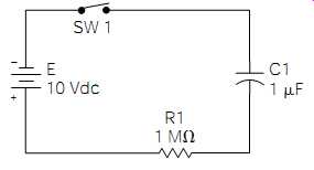
FIG. 1 Basic RC (resistive-capacitive) circuit.
Here is an analogy to help clarify the previous functional aspects of capacitor theory-electrical references will be to the circuit shown in Fig. 1. Imagine that you have a very large tank of water filled to a 10-foot level (this is analogous to the battery at a 10-volt potential). From this large tank, you wish to fill a small tank to the same 10-foot level (the small tank is analogous to the capacitor). You connect a water pipe and valve from the bottom of the large tank to the bottom of the small "empty" tank. When you first open the water valve to allow water to flow from tank to tank, the flow rate will be at its highest because the level differential will be at its greatest (the water flow is analogous to electric current flow). As the water begins to fill up the small tank, it also begins to exert a downward pressure opposing the flow of incoming water. Consequently, the flow rate begins to decrease. As the water level in the small tank gets higher, the flow rate continues to decrease until the small tank is at the same 10-foot water level as the large tank.
As soon as the two levels are equal, all water flow from tank to tank will cease. As the old proverb states, "water seeks its own level." If you were to monitor the level increase in the small tank with respect to time, you would notice that the level does not rise in a linear fashion; that is, it rises at a slower rate as it approaches the 10-foot top. If you charted the rise in "level versus time" in the form of a graph, the curve would be identical to the curve shown in Fig. 2.
The small water tank will have a holding capacity associated with it. For instance, it can be specified as capable of holding 40 gallons. Capacitors are also rated with respect to the quantity of charge they can hold.
The capacity (quantity of charge) of a capacitor is measured in units called farads. A farad is the amount of capacitance required to store one coulomb of electrical energy at a 1 volt potential. A coulomb is a volume measurement unit of electrical energy (charge). It is analogous to other volume measurement units such as quart, pint, or gallon. A gallon represents 4 quarts. A coulomb represents 6.28 x 10^18 electrons (or 6,280,000,000,000,000,000 electrons). The basic unit of current flow, the ampere, can be defined in terms of coulombs. If one coulomb passes through a conductor in one second, this is defined as one ampere of current flow. Thus, 1 amp _ 1 coulomb/second.
A farad is generally too large of a quantity of energy to be stored by only one capacitor. In the 1930s, a Gernsback magazine calculated the size requirements for building a 1-farad paper-foil capacitor. Completely fill the Empire State Building, from bottom to the top, with a stack of paper and foil layers!
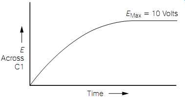
FIG. 2 Capacitor voltage response of Fig. 1.
Therefore, the capacity of most capacitors is defined in terms of microfarads (1 uF =0.000,001 farad) or picofarads (1 pF = 0.000,000,000,001 farad). As stated previously, capacitors also have an associated voltage rating. If this voltage rating is exceeded, the capacitor could develop an internal short (the term short means an undesired path of current flow. In reference to capacitors, the short would occur through the dielectric, destroying the capacitor in the process).
As the graph in Fig. 2 illustrates, the capacitor in the circuit of Fig. 1 charges exponentially. This means that it charges in a nonlinear fashion. An exponential curve (like the charge curve in Fig. 2) is one that can be expressed mathematically as a number repeatedly multiplied by itself. The exponential curve of the voltage across a charging capacitor is identical to the exponential curve of the current increase in an LR circuit as shown in Section 3 (Figs. 5 and 6).
As discussed in Section 3, the current change in an LR (inductive resistive) circuit, relative to time, is defined by the time constant and expressed in seconds. Similarly, in an RC (resistive-capacitive) circuit, the voltage change across the capacitor is defined by the time constant, and it is also expressed in seconds. An RC time constant is defined as the amount of time required for the voltage across the capacitor to reach a value of approximately 63% of the applied source voltage. The RC time constant is calculated by multiplying the capacitance value (in farads) times the resistance value (in ohms). For example, the time constant of the circuit shown in Fig. 1 would be:
Tc = RC = (1,000,000 ohms) (0.000,001 farad) = 1 second
The principle of the time constant, that applies to inductance, also applies to capacitance. During the first time constant, the capacitor charges to approximately 63% of the applied voltage. The capacitor in Fig. 1 would charge to approximately 6.3 volts in one second after SW1 is closed. This would leave a remaining voltage differential between the battery and capacitor of 3.7 volts (10 volt - 6.3 volts = 3.7 volts). During the next time constant, the capacitor voltage would increase by an additional 63% of the 3.7-volt differential; 63% of 3.7 volts is approximately 2.3 volts. Therefore, at the end of two time constants, the voltage across the capacitor would be 8.6 volts (6.3 volts + 2.3 volts =8.6 volts). Five time constants are required for the voltage across the capacitor to reach the value usually considered to be the same as the source voltage.
In the circuit shown in Fig. 1, the approximate source voltage (10 volts) would be reached across the capacitor in 5 seconds. If SW1 is opened, after C1 is fully charged, it would hold the stored energy (1 microfarad) at a 10-volt potential for a long period of time. A "perfect" capacitor would hold the charge indefinitely, but in the real world, perfection is hard to come by. All capacitors have internal and external leak age characteristics, which are undesirable. It would be reasonable, however, to expect a well-made capacitor to hold a charge for several weeks, or even months.
Consider the current and voltage relationship in Fig. 1 when SW1 is first closed (assuming C1 is discharged). Immediately after SW1 is closed, the capacitor offers virtually no opposition to current flow (just like the small empty water tank in the earlier analogy). This maximizes the current flow, and minimizes the voltage across the capacitor. As the capacitor begins to charge, the current flow begins to decrease. At the same time, the voltage across the capacitor begins to increase. As stated earlier, this process continues until the voltage across the capacitor is equal to the source voltage, and all current flow stops.
The important point to understand is that the peak current occurs before the peak voltage is developed across the capacitor. Simply stated, the voltage lags behind the current in a capacitive circuit. As a matter of convenience, professionals in the electrical and electronics fields tend to describe this phenomenon as "the current leading the voltage." This is very much akin to deciding how to describe a glass containing water at the 50% level; is it half full or half empty? As discussed in Section 3, the current lags the voltage by 90 degrees in a purely inductive circuit. In comparison, the current leads the voltage by 90 degrees in a purely capacitive circuit. As in the case of purely inductive circuits, purely capacitive circuits do not dissipate any "true" power because of the 90-degree phase differential between voltage and current.
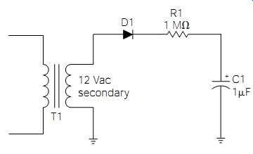
FIG. 3 A DC filter circuit.
Filter Capacitors
Capacitors used in filter applications remove an AC component from a DC voltage. Some filter capacitors are implemented to remove only a frequency-dependent part of an AC signal, but these applications will be discussed in a later section. In this section, you will examine how filter capacitors are used in DC power supply applications.
FIG. 3 illustrates a simple half-wave rectifier circuit with R1 and C1 acting as a filter network. For a moment, review what you already know about this circuit. T1's secondary is rated at 12 volts AC. This is an rms voltage, because no other specification is given. The peak voltage output from this secondary will be about 17 volts (12 volts x 1.414 = 16.968 volts). The negative half-cycles (in reference to circuit common) will be blocked by D1, but it will act like a closed switch to the positive half-cycles, and apply them to the filter network (R1 and C1). The amplitude of the applied positive half-cycles will not be the full 17 volts, because the 0.7-volt forward threshold voltage must be dropped across D1. This means that the positive half-cycles applied to the filter network will be about 16.3 volts in peak amplitude.
These positive half-cycles will occur every 16.6 milliseconds (the reciprocal of the 60-hertz power-line frequency). The positive half-cycle duration will be about 8.3 milliseconds, because it only represents one half of the full AC cycle. [Refer back to Section 4 (Fig. 5) and the related text if this is confusing.] Going back to Fig. 1, the calculated time constant for the circuit was 1 second. Because the same component values are used in the filter network of Fig. 3, the time constant of this filter is also 1 second. In power supply circuits, this time constant is called the source time constant.
Assuming that C1 is fully discharged, examine the circuit operation of Fig. 3 from the moment that power is first applied to the primary of T1. When D1 is forward-biased by the first positive half-cycle from the T1 secondary, the 16.3-volt peak half-cycle is applied to the filter network of R1 and C1. C1 will begin to charge to the full 16.3-volt peak amplitude, but it will not have time to do so. Because the filter's RC (resistor capacitor) time constant is 1 second, and the positive half-cycle only lasts for 8.3 milliseconds, C1 will only be able to charge to a very small percentage of the full peak level.
During the negative half-cycle, while D1 is reverse-biased, C1 cannot discharge back through D1; because C1's charged polarity reverse-biases D1. Therefore, C1 holds its small charge until the next positive half-cycle is applied to the filter network. During the second positive half-cycle, C1 charges a little more. This process will continue, with C1 charging to a little higher amplitude during the application of each positive half-cycle, until C1 charges to the full 16.3-volt peak potential. When C1 is fully charged, all current flow within the circuit will cease; C1 cannot charge any higher than the positive peak, and D1 blocks all current flow during the negative half-cycles. At this point, the voltage across C1 is pure DC.
The AC component (ripple) has been removed, because C1 remains charged to the peak amplitude during the time periods when the applied voltage is less. Even if all circuit power is removed from the T1 primary, C1 will still remain charged because it doesn't have a discharge path.
Notice that it could not discharge back through D1, because its charged polarity is holding D1 in a reverse-biased state.
The operation of the circuit illustrated in Fig. 3 can be compared to pumping up an automobile tire with a hand pump. With each downward stroke of the hand pump, the pressure in the tire increases a little bit.
Think of the tire as being C1. Air is inhibited from flowing back out of the tire by a small one-way air valve in the base of the pump. The one-way air valve allows air to flow in only one direction: into the tire. D1 allows current to flow in only one direction, causing C1 to charge. When the tire is pumped up to the desired pressure, it will hold this pressure even if the pump is removed. Once C1 is charged up to the peak electrical pressure (voltage), it will retain this charge, even if the circuit power is removed.
Although the circuit of Fig. 3 is good for demonstration purposes, it is not very practical as a power supply. To understand why, examine the circuit illustrated in Fig. 4. You should recognize T1 and the four diode network as being a full-wave bridge rectifier. As discussed in Section 4, for each half-cycle output of T1's secondary, two diodes within the bridge will be forward-biased, and thus conduct "charging" current in only one direction through C1. With SW1 opened, C1 will charge to the peak voltage, minus 1.4 volts (since two bridge diodes must drop their forward threshold voltages at the same time; 0.7 volt + 0.7 volt = 1.4 volts).
The peak voltage of a 12-volt AC secondary is about 17 volts, so C1 will charge to 17 volts - 1.4 volts, or about 15.6 volts. When C1 is fully charged, the voltage across it will be pure DC.
Note the symbol used for C1 in Fig. 4. The positive symbol close to one plate indicates that it is an electrolytic capacitor, meaning that it is polarized. The value also indicates this capacitor type because a capacity of 1000 uF is too large for a conventional, nonpolarized capacitor. In this circuit, the negative side is connected to circuit common, which is the most negative point in the circuit. C1 also has an associated voltage rating of 25 working volts DC (WVDC), which means that this is the highest direct voltage that can be safely applied to the capacitor. Because the peak voltage applied to it will be only 15.6 volts, you are well within the safe operating parameters in this circuit.
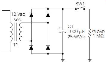
FIG. 4 Full-wave filtered DC power supply.
Referring back to Fig. 3, you calculated the source time constant by multiplying the resistance value of R1 by the capacitance value of C1.
This RC time constant was 1 second. Going back to Fig. 4, it might appear that C1 would charge "instantly" because there doesn't seem to be any resistance in series with it. In an "ideal" (perfect) circuit, this would be true. In reality, the DC resistance of the T1 secondary, the wiring resistance, and a small, nonlinear "current-dependent" resistance presented by the diode bridge will be in series with C1. Of these three real-world factors, the only one that is really practical to consider is the DC resistance of the T1 secondary.
For illustration, assume that the DC resistance of T1's secondary winding is 1 ohm. To calculate the source time constant, the 1-ohm resistance would be multiplied by the capacity of C1:
Tcsource _ (1 ohm) (0.001 farad) _ 0.001 second (or) 1 millisecond
Because the time duration of each half-cycle is approximately 8.3 milliseconds, for all practical purposes, you can say that C1 will be fully charged by the end of the first positive half-cycle. During the rapid charging of C1, a very high surge current will flow through the diode pair that happens to be in the forward conduction mode at the time.
This is because C1 will initially look like a direct short until it is charged to a sufficient level to begin opposing a substantial portion of the current flow.
As you may recall, one of the forward current ratings for diodes (discussed briefly in Section 4) was called the peak forward surge current and was based on an 8.3-millisecond time period (for 60-hertz service). The purpose for such a rating should now become apparent. Diodes, used as power supply rectifiers, will be subjected to high surge currents every time the circuit power is initially applied. 8.3 milliseconds is used as a basis for the peak forward surge current rating, because that is the time period of one half-cycle of 60-hertz AC. A rule-of-thumb method for calculating the peak forward surge current is to estimate the maximum short-circuit secondary current of T1 based on its peak output voltage and DC resistance. The peak output voltage of a 12-volt secondary is about 17 volts, and you have assumed the DC resistance to be 1 ohm. Therefore, using Ohm's law:
I peak surge
__ _ 17 amps peak 17 volts
_ 1 ohm Epeak
_ R
In reality, a transformer with a 12-volt secondary, and a secondary DC resistance of 1 ohm, would not be capable of producing a 17-amp short circuit current (remember about inductive reactance being additive to resistance), so this gives us a good margin of safety.
After the first half-cycle, C1 is assumed to be fully charged. As long as SW1 is open (turned off), the only current flow in the circuit will be a very small leakage current which is considered negligible. The voltage across C1 is pure DC at about 15.6 volts.
A power supply would be of no practical value unless it powered something. The "something" that a power supply powers is called the load. The load could be virtually any kind of electrical or electronic circuit imaginable; but in order to operate, it must draw some power from the power supply. In Fig. 4, a load is simulated by the resistor Rload. By closing SW1, the load is placed in the circuit, and the circuit operation will be somewhat changed.
In power supply design, it is important to consider the source time constant (calculated previously) as well as the load time constant. When C1 is charged, it cannot discharge back through the bridge rectifier and the T1 secondary, because its charged polarity reverse-biases all of the diodes.
By closing SW1, a discharge path is provided through Rload. The load time constant (sometimes called the discharge time constant) can be calculated by multiplying the capacitance value of C1, by the resistance value of the load (Rload:
TCload _ (0.001 farad) (1000 ohms) _ 1 second (1000uF = 0.001 farad)
The importance of the load time constant becomes apparent by examining the "exaggerated" illustration of Fig. 5. The waveshape shown in dotted lines is the 120-hertz, full-wave from the bridge rectifier circuit. As calculated earlier, this time constant is very short (only 1 millisecond). So, for illustration purposes, this charge is shown to be concurrent with the applied 120-hertz half-cycles.
The discharge periods represent the load time constant. During these periods, C1 is supplying its stored energy to power the load, causing its voltage level to drop by some percentage until the next charge period replenishes the drained energy. The variations in voltage level between the charge and discharge periods is called ripple. In a well-designed power supply, ripple is a very small, undesirable AC component "riding" on a DC level. Ripple can be specified as a peak-to-peak value, an rms value, or a percentage relationship, as compared to the DC level.
As stated earlier, the illustration in Fig. 5 is exaggerated; the ripple variations would not be nearly as pronounced, because the load time constant (1 second) is much longer than the peak charging intervals, which occur every 8.3 milliseconds. As a general rule of thumb, the load time constant should be at least 10 times as long as the charge interval. In the case of a full-wave rectifier circuit, as in Fig. 4, the charge interval is 8.3 milliseconds, so the load time constant should be at least 83 milliseconds. With a half-wave rectifier circuit, the load time constant would have to be twice as long for the same quality of performance.
The power supply illustrated in Fig. 4 is referred to as a raw DC power supply. This simply means that it is not voltage- or current-regulated. Regulated power supplies will be discussed in Section 6.
Designing Raw DC Power Supplies
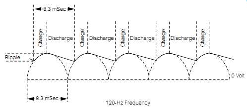
FIG. 5 Charge/discharge cycle of C1 in Fig. 4.
Every type of electrical or electronic apparatus needs a source of electrical energy to function. The source of electrical energy is called the power supply. The two main classifications of power supplies are line operated power supplies (operated from a standard 120-volt AC wall outlet) and battery supplies (electrical energy is provided through a chemical reaction). It is relatively safe to say that any device capable of functioning properly from a battery power source, can function equally well from a properly designed "raw" DC power supply, receiving its energy from a wall outlet. This is important because you will probably run into many situations where you will want to test or operate a battery-powered device from standard household power. As an exercise to test all you have learned thus far, here is a hypothetical exercise in designing a raw DC power supply for a practical application.
Assume that you own an automobile CB (citizen's band) radio that you would occasionally like to bring into your home and operate as a "base station." In addition to installing an external stationary antenna (which is irrelevant to our present topic of discussion), you would have to provide a substitute for the automobile battery as a power source. The CB radio is specified as needing "12 to 14 volts DC at 1.5 amps" for proper operation.
The CB radio power supply will have three primary parts: the trans former, a rectifier network, and a filter. You should choose a transformer with a secondary "peak" (not rms) voltage rating close to the maximum desired DC output of the power supply. In this case, a 10-volt AC secondary would do nicely, and they are commonly available. The peak voltage output of a 10-volt secondary would be
Peak _ 1.414(rms) _ 1.414(10 volts) = 14.14 volts
The rectifier network will drop about 1 volt, so that would leave about 13 volts (peak) to apply to the filter capacitor. The current rating of the transformer secondary could be as low as 1.5 amps, but a 2-amp secondary current rating is more common, and the transformer would operate at a lower temperature. A transformer with a 10-volt AC at 2-amp secondary rating can also be specified as a 10-volt 20-volt-amp trans former. The volt-amp (V A) rating is simply the current rating multiplied by the voltage rating (10 volts _ 2 amps _ 20 VA).
A full-wave bridge rectifier can be constructed using four separate diodes, or it can be purchased in a module form. Bridge rectifier modules are often less expensive, and are easier to mount. The average forward current rating should be at least 2 amps, to match the transformer's secondary rating. The peak reverse-voltage rating, or PIV, would have to be at least 15 volts (the peak output voltage of the transformer is 14.14 volts), but it is usually prudent to double the minimum PIV as a safety margin.
However, a 30-volt PIV rating is uncommon, so a good choice would be diodes (or a rectifier module) with at least a 2-amp, 50-volt PIV rating.
If you purchase these rectifiers from your local electronic parts store, don't be surprised if they don't have an associated "peak forward surge current" rating. Most modern semiconductor diodes will easily handle the surge current if the average forward current rating has been properly observed. This is especially true of smaller DC power supplies, such as the hypothetical one presently being discussed. If it is desirable to estimate the peak forward surge current, measure the DC resistance of the transformer secondary, and follow the procedure given earlier in this section. (The secondary DC resistance can be difficult to measure with some DVMs because of its very low value.) In order to choose a proper value of filter capacitance, you can equate the CB radio to a resistor. Its power requirement is 12 to 14 volts at 1.5 amps. Using Ohm's law, you can calculate its apparent resistance:
R __ _ 8 ohms (worst case) 12 volts
__ 1.5 amps E _ I
As far as the power supply is concerned, the CB radio will look like an 8-ohm load. Note that the 8-ohm calculation is also the worst-case condition. If the upper voltage limit (14 volts) had been used in the calculation, the answer would have been a little over 9.3 ohms. Eight ohms is a greater current load to a power supply than 9.3 ohms (as the load resistance decreases, the current flow from the power supply must increase).
You now know two variables in the load time constant equation: the apparent load resistance (Rload ) and the desired time constant (83 milliseconds with a full-wave rectifier). To solve for the capacitance value, the time constant equation must be rearranged. Divide both sides by R:
_ R(C)
_ R Tc
_ R
The R values on the right side of the equation cancel each other, leaving
_ C or C _ Tc
_ R Tc
_ R R R
By plugging our known variables into the equation, it becomes:
C __ 0.010375 farad or 10,375 _F 83 milliseconds
__ 8 ohms
According to the previous calculation, the filter capacitor needed for the CB radio power supply should be about 10,000 uF. A capacitor of this size will always be electrolytic, so polarity must be observed. The voltage rating should be about 20 to 25 WVDC (this provides a little safety mar gin over the actual DC output voltage), depending on availability. If this calculation had been based on a half-wave rectifier circuit, the required capacitance value for the same performance would have been about 20,000 uF.
Assembly and Testing of Third Section of a Lab Power Supply
Materials needed for the completion of this section are (1) three phenolic type, 2-lug solder strips (see text) and (2) two 4400-uF, 50-WVDC electrolytic capacitors. The phenolic solder strips are specified only because they are inexpensive and effective. If your local electronics parts store doesn't have these in stock, there are many good alternatives. Any method of providing three chassis mountable, insulated tie points that will hold the filter capacitors firmly in place, and allow easy connections to the capacitor leads, will function equally well.
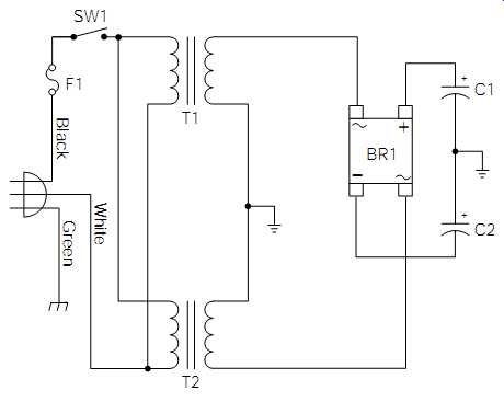
FIG. 6 Schematic diagram of the first, second, and third sections of
the lab power supply.
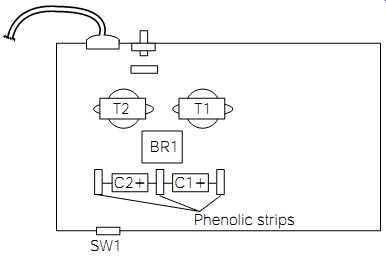
FIG. 7 Approximate physical layout of the major components for the lab
power supply project.
Referring to Figs. 6 and 7, mount the solder strips to the chassis, being careful to space them far enough apart to allow room for the capacitors (C1 and C2). Connect the capacitors to the insulated lugs and crimp the leads to hold them in place, until the remaining wiring is completed. Connect a piece of hook-up wire, from the joint connection of C1 and C2, to the circuit common point between the secondaries of T1 and T2. Use another piece of hook-up wire to connect the positive side of C1 to the positive terminal of BR1. Connect another piece of hook-up wire from the negative side of C2 to the negative terminal of BR1. Do not connect circuit common to chassis ground. At this stage of the project, the only connection to circuit common should be the junction of C1 and C2. Double-check all wiring connections, and be sure all of the voltage polarities are correct. Solder all of the connections.
The power supply you have constructed thus far is called a dual-polarity, 34-volt raw DC power supply. It is the same type of power supply as is illustrated in Fig. 4 (minus Rload and SW1). Power supplies similar to this one are commonly used in audio power amplifiers. This particular power sup ply could provide the electrical energy that a power amplifier would need to drive an 8-ohm speaker at about a 50-watt rms level. Audio amplifiers will be covered further in Section 8. Section 6 will discuss how to add an adjustable regulator section, to this design, for improved lab performance.
Testing the Power Supply
To limit redundancy, it is assumed at this point that you are practicing all of the safety procedures that have been discussed previously. In the successive sections, I will mention only the special safety considerations which can apply to unique situations. Review all of the safety recommendations presented thus far, and put them to use all of the time.
Set your DVM to measure "DC volts" on the 100-volt range (or higher).
Plug the power supply into the outlet strip. Set SW1 to the "off" position and turn on the outlet strip. Briefly, turn SW1 to the "on" position, and then back to the "off" position. Turn the outlet strip off. Measure the DC voltage across C1 and C2, paying close attention to the polarity (C1 should be positive, and C2 should be negative, in reference to circuit common). The actual amplitude of the voltage is not important at this point in the test.
You have simply "pulsed" the power supply on and off, to verify that the capacitors are charging and in the correct polarity. As you measured the DC voltages, they should have been decreasing in amplitude as the charge was draining off. The draining of the charge is caused by the internal leakage inherent in all electrolytic capacitors (new capacitors can be very leaky until they have the chance to re-form during circuit operation). Also, the capacitors will discharge, to some degree, through the internal input impedance of the DVM while you are measuring the voltage.
If you measured some voltage level across C1 and C2, with the correct voltage polarities, reapply power to the circuit and measure the DC voltages across C1 and C2. The calculated voltage across each capacitor should be about 33 volts (the peak value of the 24-volt secondaries is about 34 volts, minus an estimated 1-volt drop across the rectifier). In reality, you will probably measure about 36 to 38 volts across each capacitor. There are several reasons for this higher level. Transformer manufacturers typically rate transformers based on minimum worst-case conditions, so it is common for the secondaries to measure a little high under normal conditions. Also, you are measuring the voltage levels under a no-load condition (often abbreviated N.L. in data books). If you took these same measurements while the power supply was operating under a full load (abbreviated F.L.), they would be considerably lower.
Leaving power applied to the power supply circuit, set your DVM to measure "AC volts" beginning on the 100-volt (or higher) range. Measure the AC voltage across C1 and C2. If you get a zero indication on the 100 volt range, set the range one setting lower and try again. Continue this procedure until you find the correct range for the AC voltage being measured. (When measuring an unknown voltage or current, always begin with a range setting higher than what you could possibly measure and work your way down. Obviously, if you are using an "autoranging" DVM, you won't have to worry about setting the range.) If the circuit is functioning properly, you should measure an AC component (ripple) of about 5 to 20 mV. Turn off the circuit.
Many of the more expensive DVMs are specified as measuring true rms. If you are using this type of DVM to measure the ripple content, the indication you'll obtain will be the true rms value. The majority of DVMs, however, will give an accurate rms voltage measurement of sine-wave AC only. Referring back to Fig. 5, note that the ripple wave shape is not a sine wave; it is more like a "sawtooth" (you'll learn more about differing waveshapes in succeeding sections). The point here is that there can be some error in the ripple measurement you just performed. High accuracy is not important in this case, but you can experience circumstances in the future, where you must consider the type of AC waveshape that you are measuring with a DVM, and compensate accordingly.
As an additional test, I used a 100-ohm, 25-watt resistor to apply a load to the circuit. If you have a comparable resistor, you might want to try this also, but be careful with the resistor; it gets hot.
The resistor is connected across each capacitor, and the subsequent AC and DC voltage measurements are taken. The loading effect was practically identical between the positive and negative supplies, which is to be expected. The DC voltage dropped by about 3.1 volts, and the ripple voltage increased to about 135 mV. These effects are typical.
Food for Thought
Throughout this section, I have followed a more traditional, and commonly accepted, method of teaching and analyzing capacitor theory.
I suggest that you continue to comprehend capacitor operation from this perspective. However, in the interest of accuracy, you will find the following story to be of interest.
Michael Faraday, the great English chemist and physicist, had a theory that more closely approaches the way a capacitor really works. His theory stated that the charge is actually contained in the dielectric material--not the capacitor's plates. Inside the dielectric material are tiny molecular dipoles arranged in a random fashion. Applying a voltage to the plates of a capacitor stresses these dipoles causing them to line up in rows, storing the energy by their alignment. In many ways, this is similar to the physical change occurring in iron, when it becomes a temporary magnet by being exposed to magnetic flux lines. When a capacitor is discharged, the dipoles flex back like a spring, and their energy is released.
The fact that the stored energy within a capacitor is actually contained within the dielectric explains the reason why different dielectric materials have such a profound effect on the capacity value.
Dielectric materials are given a dielectric constant rating (usually based on the quality of air as a dielectric; air _ 1.0) relative to their overall effect on capacity. A dielectric material with a rating of 5, for example, would increase the capacitance value of a capacitor to a value 5 times higher than air, when all other variables remained the same.