There is evidence from studies of the brain that the perception of music is different from the perception of language, and that words which are spoken are perceived differently than words which are sung. There is also evidence that the way in which we perceive certain natural sounds, whether as music or language, may be related to cultural differences and learning experience. If these, and many other such things in our perception of sound, be true, then where in our audio technology do we address such factors? If not, then why not?
In an earlier discussion, I broached the issue of the end product of audio.
The end product is the listening experience. The end product is not advertising specs, it is not meter readings, or wiggles on an oscilloscope, or piles of charts and graphs. The end product is that very private and personal experience we have when listening to reproduced sound.
If we are ever going to put a number, on the quality of that experience, then it is clear that we must do more than specify the cosmetic perfection of a waveform or pursue an endless quest of reducing measurable distortions on laboratory signals which may have little bearing on the process of perception of sound.
Somehow in our technical considerations of audio we must also recognize the role played by human emotion.
Aggression, paradox, strength of opinion, and conflict of interest may not be considered as control variables by an audio designer, but they can be very important in determining the success of the product which he designs.
Under The Lamppost
Achieving a satisfactory illusion of reality is a goal of present audio technology. But understanding how to achieve this goal demands that we consider a great deal more than some of us may be willing to admit. I know from firsthand experience the feelings of frustration that can result when an audio component measures well but sounds bad. Fancy mathematics and precision test equipment tend to lose their charm when they disagree with our ears.
The problem lies not in our science but in ourselves. We misapply the science. Nowhere is this more evident than in the way in which we use concepts drawn from linear mathematics to develop models of distortion.
Today's best distortion measurements are based on linear theory. Need we wonder why it does not always work? A suitable parable for this misapplied attitude can be found in an old theater routine. The curtain opens to show a man, obviously well in his cups, muttering incoherently and scrambling around on his hands and knees under a lamppost. Soon a policeman strolls by, looks at the drunk's frantic motions, and asks the cause of his actions. The drunk replies that he dropped his last coin and must find it since it was his carfare home. So the kindly peace officer gets down on his own hands and knees and commences to help look for the coin under the lamppost. After a while, the policeman asks if the man is sure he dropped the coin in this place. "No," the drunk replies, "I dropped it over there," pointing to the dark bushes away from the post. "What," the policeman bellows, "are you doing looking for it here?" "The light is better here," answers the drunk.
That corny old stage routine is a good analogy for many of the things we tend to do in the name of science.
We solve the linear math problem be cause the light is better there. And, just like the man in his cups who can justify his deeds because he can see what he is doing, we can produce dazzling mathematical chicken tracks to defend our choice of mathematics.
But it is not the mathematics that is wrong; the folly lies in its misapplication. Nor can we excuse our use of linear concepts by assuming that a so called "piecewise linear" approximation will always work for nonlinear situations. It won't always work. And where it fails the worst is in the most interesting type of distortion of all distortion giving rise to instability of form.
Instability is a most important consideration in audio, particularly as it relates to our perception. When an amplifier is unstable, we consider it a bad amplifier. Our perception of sound quality can also be unstable, but unstable perception is not considered bad perception. We accept that a sound system can sound great for some type of material and terrible for others. Our opinion of a sound system can change dramatically, but we seldom think there might be some underlying pattern of behavior which, if better understood, could help us understand why it sounded good one minute and bad the next. Nor could our preoccupation with linear lamp-post math ever lead us to believe that there could be a branch of mathematics which could be applied to problems of perception and to problems in equipment design.
All of this is a lead into the subject I would like to present for your consideration.
Jumping
Let us think in terms of what I shall call factors and response. Factors control response. As the controlling factors of a process smoothly change we may find that the response to those factors suddenly changes. There is a jump in response, and there may even be a jump to a new type of response.
Jumping is a property that shows up for certain types of distortion and non-linearity, and is not something handled by our present linear audio math, no matter how impressive the pedigree of that math may seem. Jumping is a manifestation of instability of form.
The split which we get when we jump from one response to another is called divergence. A relaxation of the controlling factors back to the values they had before the jump will not generally produce a backward jump in response. Usually the factors must be substantially reduced before the back ward response jump occurs. This means that if there is a jump--if there is an instability in the nonlinear process--three additional properties will appear. These are the properties of hysteresis, bi-modality, and inaccessibility.
Hysteresis is the name given to the lag in response under cyclic changes in factors which control that response. In the hysteresis region between jumps the response has an "either-or" nature -- it is bi-modal.
The response jumps from one state to another state and there is no possibility of finding a response between these two end states--the region is inaccessible.
These properties of jump, divergence, bi-modality, hysteresis, and inaccessibility are interrelated such that the appearance of one of them usually means that the others are around.
Nor are these the only properties of a nonlinear process which are not revealed when we attempt to use linear math (because the light is better there). Irreversibility is one such property. Once we jump, or cross some decision threshold, it may never be possible to get back to the original response, no matter how the factors change.
Splitting is another nonlinear property. Splitting is an ambivalence in response under certain combinations of conflicting factors. It is a coexistent response state.
Indeterminacy is a property like splitting, but more diffuse in nature.
Not an "either-or" state, indeterminacy could be characterized as a "maybe" state. Indeterminacy is an amorphous response.
Catastrophe Theory
Evolution and change. Genesis. Structural stability with preservation of form, then sudden catastrophic change.
I doubt if there is any aspect of human endeavor that does not involve the development or unfolding of circum stance. We develop rules and expectations concerning the outcome of an evolving process; and then, suddenly, there may be a surprise. Perhaps the surprise is a part of a grander set of rules which we had not anticipated, or possibly it is a sudden switch to a new set of rules--like a train being shunted onto a different set of tracks.
The concept of stability has concerned mathematicians for a long time. But it was not until the 1960s when the brilliant mathematician, Rene Thom, perceived that sudden changes in form--catastrophes--could be classified in a finite number of ways. Up until that time there seemed to be no way to put a handle on the problem. Thom was able to show that a stable unfolding of a pro cess near a point where change can occur, can have any change that does occur categorized as one of a few basic types. Thom called these elementary catastrophes.
Even in its elementary form, Catastrophe Theory stunned applied mathematics. Suddenly (a catastrophe in its own right) a nonlinear theory was available which correctly modeled processes evolving in the four dimensions of space-time. Whereas a truly original mathematical concept may re main hidden for decades until a need is found for it, Catastrophe Theory was an instant success and has been applied to disciplines as diverse as biology, economics, human behavior, and mechanical structures.
In fact the fantastic success of Catastrophe Theory has almost killed it. In a manner well known in high fidelity circles, a new idea can be picked up by overzealous proponents and trumpeted as the final breakthrough of break throughs and grandly applied to everything from toenails to tweeters. The voice of Thom has almost been drowned out by those who would take parts of this still-evolving theory and apply it indiscriminately; then reject the whole thing when it may not seem to work in certain applications.
Catastrophe Theory can, with caution, be applied to certain fundamental problems of audio and our perception of audio quality. Being a genuine mathematics of nonlinear processes, we can expect to apply it not only to physical equipment but also to our perception. But PLEASE. Catastrophe Theory is only one of several evolving mathematical concepts. While it can explain certain things that we know happen in audio, but which seem to make no sense in terms of our linear math, and it can do this in stunningly simple fashion, Catastrophe Theory is not going to be the end-all for under standing audio. Let us not make it an ad copy "zip phrase." We have quite enough of that nonsense going on now without making it worse.
In this brief discussion I want to introduce the concept of Catastrophe Theory to audio. All I can present in the short space available for such a discussion is a simple, almost naive, look at how it can be applied. My intent, as always, is to stimulate thought. In what follows I will attempt to explain the mathematical basis in terms which I hope will be understandable.
Factors--Response
Factors control response. In discussing the nature of a response (also called a behavior or reaction) we want to know those conditions under which the response has stabilized when the controlling factors are steady. We want to try to understand the response that has no tendency to drift when the controlling factors are held constant.
This will occur when the response is in those stable locations in which there is no attraction capable of pulling it away. Translated into mathematical language, the behavior pattern experiences no gradient in response when each possible control factor is held constant.
The behavior lies at a stationary point (either a minimum or point of inflection) in some sort of a response potential. The potential can be expressed as an equation in which the response is the independent variable and the control factors are coefficients. If, for example, there are two controlling factors and one type of response, the potential will be an equation in one variable with two coefficients. The condition that the gradient of this potential be zero means that the slope of this equation, with respect to the response, be set equal to zero. The set of relationships such that the gradient of the response potential is zero will define a special type of topological surface called a manifold. This manifold defines the location of all possible stationary responses.
For two factors and one response we have a three-dimensional behavior space. The manifold will be a two-dimensional surface that folds and curves through this three-dimensional behavior space.
While this may sound highly complicated, it is actually a reasonable way of conceptualizing the interaction of response and control factors. Normally, the math would stop here because we might think that there are a hopelessly large number of manifolds which could correspond to all possible situations. But Rene Thom proved a brilliant theorem that broke this problem wide open. He proved that the only possible potentials were derived from a universal unfolding of a finite number of forms. These forms are what the mathematicians call "germs of singularities." It wasn't an infinite number of surfaces after all, but a very few; and these were of known type.
The concept of germ and of unfolding is much too complicated to go into in this discussion, but the results can certainly be appreciated.
If the number of control factors is five or less, then there are only a few types of potential which will deter mine the response to those factors.
The dimension of the response manifold, derived from these elementary potentials, is always equal to the number of control factors. The way in which the response will be observed in terms of the set of control factors is a special type of mathematical map from the manifold's surface onto the space of control factors. This map is called a projection. In naive terms we could think of the projection as the shadow which the manifold response curve casts on the control space. This map, induced by the projection on the control factor space, is called the catastrophe map of the behavior potential.
Thom proved that any singularity (wild change) in the catastrophe map is equivalent to one of a finite number of types which he called elementary catastrophes. In any dynamic system there are a precise number of topologically distinct discontinuities which can occur. The number of elementary catastrophes depends only on the number of control factors, when there are five or less. For five factors, there are 11 types of elementary catastrophe.
For four factors, there are seven types; for three factors, there are five types; for two factors, there are two types; and for one factor there is only one type of elementary catastrophe which can occur. For six and above, there are an infinite number of catastrophes.
If we stop, for a moment, to think what this might mean in audio terms it gets pretty interesting. Do we like the sound of a certain loudspeaker or don't we like the sound; that, of course, is a response. What are the conflicting factors which might be involved in creating that response? Here, you can put in your own set, but suppose there are only two conflicting factors: how much we listen to live music, and how much we listen to music reproduced from this loudspeaker. The solution of this audio problem will involve the Cusp Catastrophe.
Cusp Catastrophe
If that is the ball game--two factors and one response--then there are only two kinds of elementary behavior we can expect. The names given to these are the fold catastrophe and the cusp catastrophe. Of the two, the cusp catastrophe is the more interesting from the standpoint of the behavior pattern which it predicts. In order to understand how it can be applied to this audio problem, it is necessary to continue a bit more with the basic math discussion.
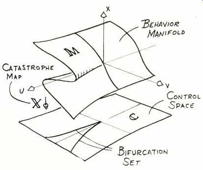
Fig. 1--When there are two control parameters, u and v, and one response,
x, the surface of stable response lies on the two-dimensional behavior manifold, M.
Let us take the case of two factors and one response and show how the cusp catastrophe develops. The potential for this particular case is the universal unfolding of a germ which is the response coordinate raised to the fourth power (that fact is not obvious nor does it follow from anything in our discussion, but is included for completeness). This potential has the form of a fourth-order equation in response with two parameters. The parameters are the coordinates of the control factors. The equation of this potential, which we shall call P, is:
P=(1/4)x4 + (1/2) u x2 +vx
where x is the response coordinate and u and v are the control factors giving rise to the response.
The response will be stationary for those values of x, u, and v where the derivative of P with respect to x is zero.
The response, in that case, will be at a stable point of the behavior potential.
This occurs when:
X2 + u x + v = 0
The two-dimensional manifold, which we will symbolize by the letter M, is then that surface in the three dimensional x, u, and v space which is described by the equation we have just developed.
If we put this manifold in the three dimensional x, u, and v space we will get the folded surface shown in Fig. 1.
This is perhaps the most widely publicized example used to describe Catastrophe Theory. The reason is because, being a two-dimensional surface in a three-dimensional space, it can be sketched and its geometry readily grasped. Like everyone else, I am guilty of showing this because it is both easy to draw and understand. There is no convenient way of sketching a three dimensional swallowtail catastrophe in a four-dimensional space, or any of the other higher-dimensional geometric catastrophe sheets.
In Fig. 1 the first thing we note about the manifold M is that for values of control parameter u above a certain level, the sheet becomes folded. The projection of this fold onto the two dimensional control space, shown as the surface labeled C, is a sharp pointed curve which forms a cusp. The projection of values found on M onto the plane C is the catastrophe map of the behavior potential. The catastrophe map is symbolized here by the capital X. Capital X, the catastrophe map, de notes the operation of dropping perpendicular projections of what is happening on M onto the plane C.
All highly symbolic, and, in typical math fashion, is shrunk down to stylized chicken tracks pregnant with meaning. But don't get hung up on the symbols or the fancy names. Think of the actions which give rise to those things. The surface M is the hypothetical manifestation of the position of unchanging response, x, under con trolling factors u and v. We, who attempt to observe the response in terms of controlling factors, cannot see the surface M. All we can observe is what happens in terms of those controlling factors. We must observe what hap pens on the surface C. We see the projection of M onto C. We see the shadow of the bird flying overhead, but not the bird itself.
The projection of the fold onto C forms two intersecting segments called the bifurcation set. The term bifurcation relates to two-forked or dual transition behavior. The cusp lines show the thresholds for sudden and catastrophic response changes which occur under action of the controlling factors. This is what gives rise to the name cusp catastrophe for the kind of behavior change we will observe.
When we change the control factors and a response is induced...and a response is induced, this is mathematically equivalent to our moving from one place to another on the manifold M. But because the point on M is controlled by changes in coordinates u and v, the point must jump whenever the increment in control passes a cusp boundary corresponding to the passage of a fold. This can be visualized by referring to the simple sketch of Fig. 2. The trajectory of response induced by a certain change in control factors is shown as curve R.
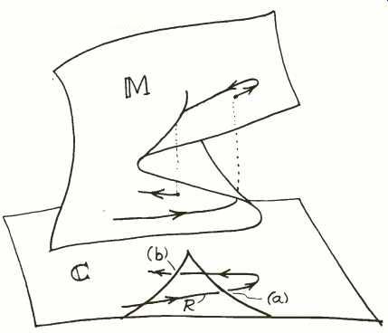
Fig. 2--Response, R, must take an abrupt jump whenever the control factors
drive behavior past the folds in the behavior manifold, M.
The place on surface M where the response occurs is found by projecting a perpendicular, upward from the corresponding u and y coordinate location, to the place where it intersects the surface M. When the control locus passes the bifurcation line at point (a), the point projected on M must jump from the lower sheet to the upper sheet as shown in this sketch, looking at the three-dimensional geometry, it is obvious what happens: In order to remain on the stable surface M, the response point must jump the gap whenever the control factors go past the fold.
But, looking at the result only in terms of the control plane C, we would see a seemingly bizarre behavior: The response was continuous and well-behaved as the factors were changed, then all of a sudden without warning the response dramatically jumped to a new behavior.
If we try to restore the original response by relaxing the control factors back to the value they had before the jump, we would not see the response come back to its former value. Instead, we would have to continue reducing the control factors back to the place where they cross the bifurcation line at (b). Then all of a sudden the response pops back to its former value. Of course, what is happening is that the trajectory on M comes back over the upper sheet until it falls over the edge of the fold, and then it is back on the lower sheet.
Flatland
If you remember one of our earlier discussions (Audio, Feb., 1979, "A View Through Different Windows"), surface C is like a Flatland. A flatlander, living on C, knows only that there are magic lines which change the way people act when passed in one direction, but which cause no change when passed in the opposite direction. A higher dimensional being can observe the surface M and comprehend why a flatlander observes a seemingly magic boundary. But any attempt to convey this fact to a flatlander will be fruitless unless the flatlander is willing to accept the reality of dimensions above those of the world which he sees.
And there is a lesson here for us. For we, too, are flatlanders who sense pat terns of response under conditions of varying factors. We can "see" the external factors and their relevance to the situation at hand. And we can ob serve how a dynamic system responds to those factors. But the hyper-surface of behavior control is invisible to us.
We sense the effect, but not the control. What Rene Thom has done is bring a higher dimensional concept to we flatlanders who could observe catastrophic changes in response, but could not reason why they should occur.
If we look at the behavior predicted by even this simple cusp catastrophe it is obvious that the properties we discussed earlier (jump, divergence, bimodality, hysteresis, and inaccessibility) are handily explained. In our next discussion, let us apply this new theory to audio.
References
1. R. Thom, "Structural Stability and Morphogenesis" (W. A. Benjamin, Reading, Mass., 1975).
2. Th. Brucker & L. Lander, "Differentiable Germs and Catastrophes" (Cambridge University Press, Cambridge, 1975).
3. Yung-Chen Lu, "Singularity Theory and an Introduction to Catastrophe Theory" (Springer Verlag, New York, 1976) .
4. E. C. Zeeman, "Catastrophe Theory, Selected Papers" (Addison-Wesley Publishing Co., London, 1977).
5. A. Woodcock & M. Davis, "Catastrophe Theory" (E. P. Dutton, New York, 1978).
6. T. Poston & I. Stewart, "Catastrophe Theory and its Applications" (Pitman, London, 1978).
Also see: Catastrophe Theory and its Effect on Audio (Part II) (Apr. 1979)
Catastrophe Theory and its Effect on Audio--Part 3, by Richard C. Heyser (Apr. 1979)
A View Through Different Windows by Richard C. Heyser (Feb. 1979)
(Source: Audio magazine, Mar. 1979; Richard C. Heyser)
= = = =