|
|
Build this versatile DIY oscillator...
This oscillator unit is capable of 0.5Hz-30kHz in one exponential (1 octave/volt) sweep and provides sine and cosine outputs (90 degree quadrature) with THD low enough ( 0.1%) for frequency response measurements and audible distortion evaluation.
ADDITIONAL FEATURES
1. THD is mostly 2 and 3 harmonic (inaudible).
2. Linear and exponential frequency control (and modulation) inputs respond cleanly with fractional-cycle response time.
3. Linear (sawtooth) sweep genera tor provides constant octave/second sweep ±1%, 20Hz-20kHz.
4. Warble (FM) generator with 0.2-10Hz rate and 0 to ±1 octave frequency deviation.
5. Stable amplitude and frequency.
OUTPUTS
Figure 1 shows the sine and cosine outputs (Fig. 1A), and their precise 90° relationship (Fig. 1B). Figure 4 shows how controlled distortion can be introduced by self-modulation (auto-FM).
CONSTRUCTION
Photos 1-3 show the unit in an 8” x 6” x 3” plastic Radio Shack project box. The circuitry (not shown) is on three solder-less breadboards containing the oscillator and auxiliary functions. Also included (not essential to the features listed) are a sweep-position meter, sweep/manual switch, 1/3 octave step switch, 10-turn fine-tune pot, and Ni-Cd batteries (not used in 13 years).
OSCILLATOR CIRCUIT
The oscillator (Fig. 2) is basically a state-variable filter (biquad) using the method I described in a 1971 Audio Engineering Society paper (“A Combination-Filter”). The “filter” is made to oscillate by having controlled positive feedback (instead of the usual negative) around the (as a filter) bandpass loop. This positive FB initially gives the “filter” a “negative Q” but is then (quickly) exactly balanced by a variable amount of negative FB, proportional to the square of the output amplitude. Thus, the “Q is made to effectively “hover at infinity,” resulting in stable oscillation.
The active gain-control elements are in T1-3, each a dual “operational trans conductance amplifier” (OTA), the Harris CA3280AE. Each section consists of an emitter-coupled bipolar diff-amp with current-mirrors, providing a push- pull Class A current source output. The transconductance (ratio of output current to base-to-base input voltage) is varied in proportion to a negative sup ply-referenced current input, which is “mirrored” to control the input diff amp’s combined emitter current.
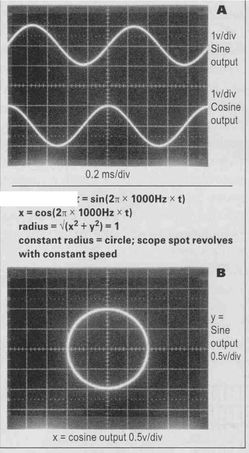
FIGURE 1A: Oscillator outputs, 1kHz.; FIGURE 1B: c = sin(2n x 1000Hz x t)


ABOVE: Photos 1-3
This control current, called ABC (Amplifier Bias Current), at pins 3 and 6 (for the two independent sections), can vary the overall transconductance by over a million to one (120dB).
Normally, an emitter-coupled bipolar transistor has a nonlinear (hyperbolic tangent) and temperature-dependent transfer curve, its “S” shape similar to the transfer of a cathode-coupled (“long tailed pair”) tube stage. However, current applied to pins 1 and 8 (the two sections) biases on a pair of back-to-back “pre-distortion diodes,” whose transfer curve and temperature dependence are inverse to those of the duff-amp (if the differential voltage inputs are sourced through a high resistance compared to 52mV/diode bias current). Then the overall transfer is very linear and temperature stable.
CIRCUIT OPERATION
OTA units Ti-A and Ti-B control the gains of integrators U1-D and U1-C, cascaded in a feedback loop. The polarity appears negative, but is made positive at the oscillation frequency with unity gain by the -180 degr. phase shift of the two cascaded integrators. The feedback is through R5 to T1-A pin 16.
In a perfect world this alone would generate a stable oscillation. But in the real world, stability must be enforced — humanity needs police, and oscillators need stabilizers (as do airplanes — we definitely don’t want them to oscillate!).
STABILIZATION LOOP
Here’s where things become interesting. Oscillators have used the variable resistance of light bulbs (slow response) or FETs, or diodes (distortion). I use T3-A, another OTA, to control negative FB around the first integrator (U1 D). A small amount of positive FB (to get things going at turn-on) is applied through R7 to T3-A pin 13 (remember that it has a current-source output, so a signal current can be summed into it to add to its load voltage).

FIGURE 2 Osc. schematic

FIGURE 2B
Notes: 1. All resistors except R33 = 1%, 1/10W or more.
2. R33 precision resistor co. PT146 ( Largo, Florida).
3. C2, C3 must be high Q, such as silver mica (not ceramic).
4. R33 and Q1 should be glued together.
Negative (damping, or in this case, growth-limiting) FB is controlled with the ‘ input (pin 3) of T3-A. But how is the signal amplitude determined? Oscillators (the ones having a feedback- control element) often use a signal “envelope follower” such as a diode-capacitor peak detector. But their output ripple must be strongly lowpass-filtered to avoid modulation distortion introduced by the FB-controlling element. The required ripple filtering makes the amplitude-stabilizing response very slow, and its time lag can even make the loop unstable.
In this oscillator, the presence of 90-degree shifted sine and cosine outputs virtually “shouts out” a solution: Those who didn’t sleep through high school trigonometry might remember that the sum of a sine squared plus a cosine squared (if of the same amplitude and the same angle or time function) equals one (unity or in this case, pure DC).
I use T2-A/EJ1-A and T2-B/U1-B as analog multipliers to square the cosine and sine outputs, respectively. Summing these squared outputs yields a signal (current in this case, feeding T3-A pin 3, the NFB control input) that is 1) virtually ripple-free DC, and 2) proportional to the square of the signal amplitude. The constant radius (circle) in Fig. 1B demonstrates the trigonometric relation ship, discovered by Pythagoras in ancient Greece.
It works very well: Upon power turn-on, the oscillator “warms up” (stabilizes) in a few cycles’ time. Once stabilized, the frequency can be square-wave modulated even from 20Hz to 20kHz, within a fraction of a cycle, without any transient “hiccupping,” and so on. The output amplitudes are about 1V RMS.
Note that the outputs of U1-A and U1-B provide, respectively, cosine squared and sine squared signals. These form a 180°-shifted pair of mostly double the oscillator frequency (with a small amount of its fundamental due to un avoidable imbalances), riding on a DC offset due to the squaring function.
OUTPUT LEVEL CONTROL
The sine and/or cosine outputs can drive a 1 to 100k log pot, with a knob that can be calibrated in V RMS, dB, and so on. I use a dual stereo 10k pot to equally attenuate the two outputs (quadrature stereo drive is described later in “oscillator applications,” no. 3).
EXPONENTIAL FREQUENCY CONTROL
In the lower left area of Fig. 2A, a matched PNP pair (Q1) is used to precisely implement the well-known exponential relation between a bipolar transistor’s collector current and base-emitter voltage. Through feedback, U2-C holds the current through the lower Q1 transistor constant, providing a 1st order VBE matching reference for the upper transistor. The latter is fed, at its base, an attenuated and temperature-compensated (by R33) frequency-control voltage, proportional to the voltages summed by U2-A.
The exponential (uniform octave; doubling per summed control volt) output current from the upper Q1 unit is divided equally by R13, Ri4 to control, by means of T1-A and Ti-B, the gains of integrators U1-D and U1-C. The oscillation frequency is proportional to the Q1 output current, and therefore is exponentially related to the summed frequency control voltages.
 FIGURE 3: Sweep and warble generators.
The 1 octave/volt scale factor has a nonlinear deviation of ±3%, from 0.4Hz to 25kHz, a range of 16 octaves. The unit, if pushed, can sweep from 0.3Hz to 50kHz. Temperature drift is about 0.2%/° C, meaning a temperature change of 300 C (540 F) causes a change of 6%, about one semitone (the 12 root of 2 = 1.059463094).
LINEAR FREQUENCY CONTROL
Applied through R42, a voltage applied here varies the collector current of the lower unit of Q1, the exponential generator’s reference current. Note: For the best temperature stability, you should mount R33 next to Q1, preferably epoxied or glued together.
SWEEP GENERATOR
This provides a linear sawtooth ramp of zero to +5V, which when fed to the oscillator's sweep input (its R37) sweeps it 10 octaves, e.g., from 20Hz to 20kHz. In Fig. 3, U1-A is an integrator (with C1) which is fed an adjustable DC current from P1 and R2. in the center ("sweep") position of Si, the output of U1-A linearly rises from zero until it reaches +5V.
Then, U1-B, a comparator with small positive FB (R10, I1) and biased to +5V (R12, R13), switches its output from about -9V to about +9V.
This turns on FET Q2, which quickly discharges C1, resetting the output of U1-A back to zero, and the cycle repeats.
With S1 in the "Lo" position, Q2 is held on, keeping U1-A output at zero, which keeps the oscillator frequency at its lowest frequency that was swept.
With S1 in the "HI" position, FET Q1 is switched across C1 through R3, R5. This keeps the output of U1-A at +5V, keeping the oscillator frequency at its highest frequency that was swept.
WARBLE GENERATOR
U1-C and U1-D make up the common triangle/square oscillator, with a range (selected by P3) of 0.1 to 10Hz. The triangle output (about ±4.4V) is adjustably attenuated by P4. The lowpass filter (R18, C4) rounds the triangle-wave peaks so that the waveform approaches a sinusoidal shape above around 5Hz (a typically useful and musically pleasing vibrato rate).
In practice, I've found this variable (with warble rate) wave shaping to be very practical: at low rates-for example, 1Hz-the triangle shape provides a linear (on a per octave basis) up and down sweep, useful for listening to speaker response variations, standing waves, and so on. But for smoothed response RTA measurements (and listening), rates around 5Hz 1) sound musically pleasing, arid 2) provide nice measurement smoothing when the oscillator's frequency deviation is 1/6 or 1/3 octave peak-to-peak, adjustable with P4.
- - - - - - -
FREQUENCY TRIMMING
1. Connect either the sine or co sine output to a frequency counter. Set P1 (coarse tune) and P2 (fine tune) to approximately center. Connect a DC voltmeter to the output of U2-i (pin 1), negative meter lead grounded.
2. Turn on the ±10V power supply. The counter should show some midrange frequency (between 200Hz-2kHz). If not, some thing is wired wrong. If or when it oscillates, proceed.
3. Adjust the coarse- and fine—tune pots to obtain zero volts ±0.01V at U2-1 pin 1.
4. Allow at least five minutes to stabilize warm-up drift. Then record the frequency
5. Adjust the coarse- and fine-tune pots (clockwise initially) to obtain negative 2.00V ±0.01V at U2-1 pin 1.
6. Adjust TP1 (1 octave/V trim) to obtain a frequency that’s four times that recorded in step 4, as closely as is practical.
7. Remove the DC voltmeter positive lead from U2-i pin 1, and connect it to the viper of P2 (fine tune).
8. Adjust P2 for zero volts ±0.1V at the wiper.
9. Set P1 (coarse tune) fully CCW.
10. Adjust TP2 (frequency trim) for 20Hz, or any other sweep-starting frequency of your choice.
11. Set P1 (coarse tune) fully CW. The frequency should be close to 20kHz, or 1000 times the lowest frequency selected in step 10.
12. You can perform back-and-forth fine tuning of TP1 and TP2 to obtain -more precision if needed.
- - - - -
OSCILLATOR APPLICATIONS
The THD of about 0.1% disqualifies it for distortion measurements. But the pure Class A analog methodology produces a "tube like" spectrum, mostly 2 and 3 harmonics. By all accounts this is inaudible, so the oscillator is perfectly acceptable for auditory evaluations and response measurements.
1. RTA (Real Time Analysis)
Measurements:
Using a sweep oscillator to display frequency response can produce accurate results, but there are two drawbacks.
First, a log converter (linear voltage to dB) is needed, along with an X-Y storage scope or chart recorder. This is virtually obsolete and cumbersome compared to computer programs such as Missa, Clio, and so on. Second, for speaker responses, in-room measurements without software "windowing" are strongly influenced by room acoustics; furthermore, a flat in-room response is undesirable because narrowing speaker dispersion and increasing room absorption at high frequencies reduce integrated response, whereas (except in the bass) you judge spectral balance primarily on the speaker's direct, "first arrival" signal.
However, listening to a swept response, or a fixed center frequency with warble, is very revealing of standing wave pat terns and speaker anomalies.
I'd like to mention that you can use a sound level meter close to a speaker (say 1m) and obtain a reasonable measurement. However, the popular Radio Shack 33-2055 meter has a broad 8dB peak around 6kHz and a rapid rolloff above 12kHz. This meter (in “C” weighting) is flat within ±1dB only from 60Hz to 1.6kHz. The Panasonic WM-60AY mike capsule, such as is used in Speaker Builder’s “Mitey Mike,” is very flat over the entire audio range. (See article “A Purist Recording Mixer,” and “Mitey Mike I,”)
2. Listening Tests
A pure sine wave, useful for amplifier tests and speaker power handling, and so on, sounds perfectly boring. However, things change radically when the tone is frequency modulated (FM, warble) at, say, a 3Hz rate with a deviation of 1 octave p-p. On good headphones, or listening right next to a good speaker; you simply hear the tone quickly sweep up and down with constant loudness.
But with a colored (resonant) speaker, or a good speaker in a room with overly live acoustics, the resonances and/or standing waves “pile up” at some swept frequency spots and cancel at others. The resulting sound is “choppy”; more over, turning your head or moving about changes the “choppy” patterns. Some times you can hear all kinds of strange effects coming from different directions, similar to “The Sound Strobe”.
3. Bass/Midrange In-Room
Measurements and Listening Tests:
At these frequencies where the aforementioned dispersion-narrowing and room absorption effects aren’t significant, in-room listening and SPL measurements can be representative of musical playback sound quality.
To evaluate a two-channel stereo system, it’s desirable to have both speakers driven. However, a mono-center signal will have a 6dB increase relative to one speaker driven (if the room and locations of the speakers and listener are reasonably symmetrical) in the bass. This is because the long wavelengths add pressure-wise (analogous to voltage) in phase. On the other hand, higher frequencies, with much shorter wave lengths, will add (or cancel) due to left! right phase randomness (unless every thing is absolutely symmetrical, which is impossible except for one ear exactly centered).
This is where the 90° (quadrature) feature of the sine/cosine outputs solves the problem. Using these two outputs as a stereo pair, even the lowest bass sound sources have a relative 90° phase shift. This makes the stereo pair add up to only a 3dB increase over one speaker driven, equal to the average random power (not pressure) addition that unavoidable asymmetry imposes on the higher frequencies.
4. Self-Modulation (Auto FM) For Controlled Distortion
Figure 4 shows interesting examples of “auto FM” wave-shaping, sometimes used for tone generation in synthesizers. Here, the sine output was connected (in Fig. 4B and 4C) to a frequency control input with 2 octave/V sensitivity (R37 labeled “sweep in” in Fig. 2A).
In Fig. 4A with no modulation (for reference), the frequency is 85Hz. Note that the X-Y (Lissajous) plot is not only a circle, but it’s of uniform brightness, because the oscilloscope spot is revolving (counterclockwise) at a constant speed, 85 times per second (5100 RPM).
In Fig. 4B, note that the output excursion is ±0.5V, meaning that the “instantaneous frequency” is modulated up and down one octave. The actual (or “average”) frequency has dropped to 74.4Hz because of the “time stretched” negative waveform portion. A mechanical analogy: Driving 30 miles at 30mph obviously takes one hour. But suppose you drive the first half (l at 15mph (an “octave lower” speed), taking one hour; and then try to make up for lost time (obviously you can’t; you’ve al ready used up the hour) by increasing your speed to an “octave higher” than the original 30mph; that is, to 60mph. The second 15 miles then takes a quarter hour, so the total trip time is 1.25 hours. Your “average frequency” (speed) is 24mph, a reduction of 20%; not the same as trying to average the 15mph and 60mph (which would erroneously give 3 7.5mph). With an auto-modulated exponential frequency versus voltage oscillator, the mechanism is more complicated than in the analogy, because nonlinear time-varying feedback is involved.


FIGURE 4: Self-modulation waveforms and XY Lissajous.
Figure 4C is a more extreme example; the waveform’s ±1.3V excursions generate ±2.6 octave modulation peaks. This modulates the average 40Hz frequency (reduced as explained) for an “instantaneous frequency” excursion range of 6.6Hz to 242.5Hz, reflected in the “cuspy” shape of the (normally) sine output. There are several fascinating features of this result:
a) The X-Y plot is still circular (meaning that the relative phases of fundamental and all harmonics in the two outputs are 90°; the two output waveforms are mutual Hubert trans forms).
b) The circle’s brightness varies, being brightest at the bottom. This is because the “sine” output (vertical axis) spends a relatively long time at a negative voltage. Thus the scope spot revolves at an uneven (“jerky”) speed, slowest at the bottom. Looks like an annular solar eclipse, where the moon is farther away than normal from the earth, so its image is too small to completely cover the sun.
c) The “sine” output has a negative DC offset (-0.92V); the AC component is 0.55V RMS; total AC + DC = 1.09V RMS.
d) The “sine” output approaches a “tapered impulse” wave, while the “cosine” output approaches a linear sawtooth.
e) The two outputs have identical harmonic amplitude spectra, and sound nearly identical, except on head phones or with very phase-coherent speakers in a dry-acoustic room. Hard to believe, but it’s true.
For less extreme FM excursions, the harmonic spectrum is low-order, resembling (and sounding like) single-ended triode tube distortion; note the “sine” output in Fig. 48. This provides a method of simulating various amounts of tube-like distortion for auditory evaluations. At various frequencies, adjusting a pot (100k or so) between either oscillator output and the (normally connected to) warble input allows you to determine your distortion audibility threshold (for smooth tube-like distortion) by monitoring the output on a distortion meter or spectrum analyzer.
Table 1 is the parts list for the oscillator, while Table 2 lists the parts for the sweep and warble generators. A regulated ±10V supply is required; current draw is about ±40mA.
TABLE 1
TABLE 2
REFERENCES
1. originally designed by RCA.
2. Not a misspelling of “annual.” Means “ring-like.”
============