|
|
The first part of an extensive study on several design considerations affecting driver performance.
You know that the presence of each driver on an enclosure front panel affects the performance of the other drivers. You also know that the cabinet edges and any grille structure tend to modify the response of all the drivers. In truth, any structure near the cone of a driver—either on the front or back—can modify the response of that driver. Symmetrical structures can be particularly destructive.
Numerous publications, including Speaker Builder and audioXpress , have published articles that address these interference problems. Generally the published graphs show comparison responses for the test driver with and without the interference present. This clearly illustrates the change in the driver’s response, but does not provide any sense for exactly how the interference causes the measured response change.
The power cepstrum plot, which is sometimes also displayed in interference studies, tells you at what times there are delayed echoes of the original signal contained within the signal with interference. Even these leave you with little idea of what the “interference signal” composed of reflections and/or diffractions really looks like. This article will show you.
There are other ways to modify the response of a driver, such as changing the acoustic loading via a horn or waveguide structure. The structures studied here are believed to not change the acoustic loading, but to modify the driver’s response via reflection and diffraction.
In this article I will investigate the interference of several structures on the performance of drivers. I will show the change in the driver’s response and present plots of the interference signal that is causing the response change. I will also illustrate how, with testing capability, you can develop these interference signal plots.
HISTORY
This all started when I was again measuring damping materials for potential use as front-panel-covering materials to reduce the destructive effects of grille structures (I had earlier co-authored work on this topic). For this testing I decided on a round grille frame mounted concentrically with the tweeter. My thinking was that with such a frame all “echo” effects would occur at the same time on-axis, thus making them more easily detected. The term “echo” is used here to refer to an interfering signal that may be any combination of reflection and diffraction effects. The round grille frame decision was terrible for testing damping materials, but good in that it led to the interference signal display technique covered in this work.
The round, concentric grille frame certainly did concentrate the echoes. The test tweeter’s response was so badly destroyed that no damping material applied to the front panel had a chance of restoring a useful tweeter response. I sent a copy of the results to George Augspurger (GLA), who computed the energy in the interference signal. Even though an interference may be composed of multiple signals that are diverse in frequency and time, at each frequency you can resolve these signals to a single resultant sine wave. Based on GLA’s work, I found that I could compute and plot this resultant interference signal, which I call the composite reflection signal. For some cases, at certain frequencies, the magnitude of this composite reflection signal will exceed the magnitude of the original driver on-axis signal. Under these conditions the interference may be delivering a higher SPL signal to your ears than the tweeter!
THE ROUND GRILLE FRAME
I used the round, concentrically mounted grille frame to demonstrate the plot ting of the composite reflection signal. It also clearly demonstrates that you should not choose to use a round grille frame, or any other symmetrical grille structure, for that matter. I first examine the results as they have generally been presented in the past and compare them with the effects of the composite reflection signal.

--- Photo 1
Photo 1 shows a dome tweeter mounted in the center of the round grille frame on my test baffle testing starts before installing the grille frame. The test tweeter is a 1-½” silk dome ( Dayton #275-070). Figure 1 shows the measured 1-m on-axis response of this tweeter surface-mounted with and with out a diffraction ring. The diffraction ring (DR) is a simple device for spreading Out the diffraction caused by the faceplate of a surface-mounted tweeter The DR does smooth the tweeter response somewhat, but in this case not nearly as much as flush-mounting might do.
Figure 2 shows the power cepstrum (PC) plot for the surface-mounted tweeter without a DR, displaying a major echo group around 0.l5ms. This corresponds to a delay distance of about 2’; which is close to the 2.15” radius of the tweeter faceplate. Figure 3 shows the PC plot with the DR added, which has clearly spread the diffraction echoes out in time with a corresponding magnitude reduction. This plot led me to expect more improvement in the frequency response than in Fig. 1. I also expected the major problems from the round grille frame to start at about 0.47ms, so I decided to test without the DR, which left the time period after ½ms more free of echoes.

FIGURE 1: Responses of Dayton tweeter with and without diffraction ring.

FIGURE 2: Power cepstrum plot for Dayton tweeter without diffraction ring.
The round grille frame is 3/4” thick (height above test baffle) with a 12” ID and 14½” OD. The test microphone is back to 44’ for a valid far-field test range including all the output from the grille frame. Figure 4 shows the tweeter response (at 44’) with and without the grille frame (GF) mounted. The GF modifies the original tweeter response at some frequencies by many dB.
The PC plot with the GF (Fig. 5) shows, as expected, large echoes spread out over greater than 1 ms. In the past I have tried to relate these echo groups to the physical dimensions of the interfering structure without learning much.
In an attempt to “cure” the destruction of this GF, I covered the front panel area inside the frame with an increasing number of thin (0.042’) felt layers. I made the bottom layer oversized to cover the inside of the frame (Photo 2). From the measured responses with the various felt layers (Fig. 6), it is clear that even this much felt does not restore the tweeter response. There is, however, a bit of a mystery in Fig. 6: Why does the dip at 3.5kHz become deeper with more layers of felt? Something is going on here that can’t be determined from the frequency response or power cepstrum plots.
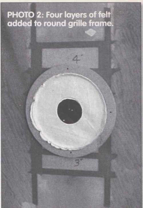
---Photo 2
THE COMPOSITE REFLECTION SIGNAL
How to implement the testing and computation to produce these plots of the composite reflection signal is covered in Appendix A For now, I will examine the test results and the composite reflection curve plots; i.e., the resultant reflection signal relative to the bare tweeter response. The basic approach is to test the frequency response of the bare tweeter and export that result as a data file. Next you add the interference object—here the round GF—and measure just the change in response, both magnitude and phase shift.
Figure 7 shows such an error plot, titled echo signal. As you can see, the amplitude variations are about 20dB peak-to-peak (PTP), and phase shift variations are up to 180-degree. These curves are also exported as a data file for computer processing.

FIGURE 3: Power cepstrum plot for Dayton tweeter with diffraction ring.
FIGURE 4: Responses of Dayton tweeter with and without round grille frame.

FIGURE 5: Power cepstrum plot of Dayton tweeter
FIGURE 6: Tweeter responses with various numbers of felt layers added.
The curves in Fig. 7 depict the changes in magnitude and phase shift that the GF would make on an “ideal” tweeter; that is, a tweeter with a perfectly flat magnitude response at 0dB and a phase shift of zero degrees. Based on these curves, your computer program can calculate the magnitude (and phase if desired) of the resultant interference signal that caused the response changes to your “ideal” tweeter. I computed only the magnitude function, calling it the composite reflection curve (CRC). You can then re-normalize the results to match your actual tweeter.

FIGURE 7: Error curves for tweeter with round grille
FIGURE 8: CRC plot for tweeter with round grille frame.
Figure 8 shows the composite reflection curve (the bold plot) for the round GF versus the bare tweeter response. The CRC is the magnitude curve of the interference that causes the measured changes in the actual tweeter’s response. It is clear that the CRC exceeds the magnitude of the tweeter response and thus, depending on phase, can cause major peaks and dips. Note that the CRC has a bandpass shape for the major interference, producing less destruction at low and high frequency. Keep in mind that while I called the CRC a reflection, its origins may be any combination of reflections and diffractions caused by the interfering object and arriving at the on- axis microphone during the FFT time window used.

FIGURE 9: Error curves for tweeter with round grille frame and four layers
of felt.
FIGURE 10: CRC plot for tweeter with round grille frame and four layers of felt.
Figure 9 shows the error signal magnitude and phase shift for the “ideal” tweeter with four layers of felt added to the GF. Both the magnitude and phase shift variations are reduced, as you would expect. The CRC plot in Fig. 10 shows that the interfering signal still nearly matches the tweeter response magnitude in the 2kHz to 4.5kHz range. It is clear that depending on the phase relation ship the GF is capable of producing the deep dip that was noted with four layers of felt.
I believe that the CRC plot adds new insight into what happens when some object interferes with a driver’s response. You see in what frequency range the major destruction will occur and how large the magnitude variations might be. I cover only on-axis testing in this article, but you can apply the same technique to off-axis testing.
A MORE RATIONAL GRILLE FRAME
I tested the same surface—mounted tweeter with a more realistic GF constructed of 1/2” x ½” bars. This half-inch- tall rectangular structure was 10” wide by 14 1/2” high on the inside and positioned as on a small two-way system. The tweeter was offset from the centerline by ¾” destroy symmetry (Photo 3).
To try and learn more about the mystery of GF diffraction, I did not install the frame all at once, but one bar at a time. I measured the effect of each additional bar on the tweeter’s response. The microphone was back 57” to provide a valid far-field response for the full GF.
The first bars installed were the top of the frame and then the left side. These two bars are nearest the tweeter, so I expected them to cause the most trouble.
Figure 11 shows the tweeter response bare, with only the top bar and with the top and left bars. There is very little destruction of the tweeter’s response.

FIGURE 11: Responses for bare tweeter, top GF bar, and top and left GF bars.
FIGURE 12: Power cepstrum plot for tweeter with top and left GF bars.
Figure 12 is the PC plot for the top and left bars with echoes out to about 3 indicated. Figure 13 shows the error curves for the case of the top and left bars installed, again showing a minimum of response change. The CRC plot in Fig. 14 shows an interference signal running about 20dB below the tweeter response from about 2kHz to 9kHz. This indicates a wide but gentle destruction of the bare tweeter response.

FIGURE 13 Error curves for tweeter with top and left GF bars.

FIGURE 14 CRC plot for tweeter with top and left GF bars.
Next I added the bottom (farthest) and finally the right bars. Figure 15 shows the responses for the bare tweeter, then the top, left, and bottom bars, and finally all four bars. To my surprise, the most distant bars cause more response destruction than the closest bars.
The PC plot for the four bars (Fig. 16) contains echoes out past 1ms. The error curves for these four bars (Fig. 17) indicate more error than for just the two closest bars. The CRC plot for the four bars (Fig. 18) shows that the interference signal magnitude has risen to the -10 to -13dB level over the range 2kHz to 6kHz, resulting in the increased bare-tweeter response destruction.
You might argue that the reason for the increase is because four bars are worse than any two. While not shown here, I tested this option by removing the two closest bars and verifying that the two furthest bars alone produce most of the destruction. I don’t really know why this is so. It may be that the faceplate of the surface-mounted tweeter masks the sound energy to the closest bars or that the longer time delay of the farthest bars causes more trouble.
Remember, I am measuring only the on-axis response destruction. It may well be that the closest bars cause more trouble off-axis. The point to remember is that all of the grille frame—not just the portions close to the tweeter—should be considered as a potential problem.
MIDRANGE’S EFFECT ON TWEETER’S RESPONSE
It is well known that when you add drivers to the front panel, you modify the response of each driver from what it was alone. I decided to investigate the changes in the response of a tweeter when a midrange driver was added. To minimize the interference, I flush-mounted the drivers, which included the Terra CS- 1.1 tweeter, an inverted 1.1” aluminum dome, and the 51%” Terra CS-4ABSE open-back midrange, which is actually a mid-bass driver, again with aluminum cone. Photo 4 shows the two drivers in the test baffle mounted at 6” center-to-center (CTC). Due to the reduced span of the two drivers, the microphone is back only 1m for a valid far-field test.
Figure 19 plots the bare tweeter response (midrange replaced with a solid panel) and the tweeter response with the midrange mounted. I w thinking “two-way system” when taking this data, so the figure mentions a “woofer,” but it is actually the 51% Terra Mid-Bass noted above. Response changes are noted from low frequency right to 10kHz, but seem worse in the 2—3kHz and 5—7kHz ranges.

FIGURE 15: Responses for bare tweeter, top, left, and bottom GF bars; and
all four GF bars.
FIGURE 16: Power cepstrum plot for tweeter with four – GF bars.

FIGURE 17 Error curves for tweeter with four GF bars
FIGURE 18: CRC plots for tweeter with four GF bars.
The error curves (Fig. 20) display slight response errors in the “ideal” tweeter response. The CRC plot (Fig. 21) shows the interference signal is down only 18—20dB in some ranges and demonstrates why the bigger response changes do occur 2—3kHz and 5—7kHz. So even with both drivers flush-mounted and fairly widely separated, the mid range can have a measurable effect on the tweeter’s on-axis response.
TWEETER’S EFFECT ON MIDRANGE’S RESPONSE
While the presence of the midrange added about ±2dB of response variation to the tweeter, would the tweeter have any effect on the midrange response? I performed this test using the same two drivers as above tested at 1m. Figure 22 presents the response of the midrange with and without the tweeter. Note that while this midrange shows the typical break-up ripple of an aluminum cone driver above 4kHz, it is actually capable of a smoother response below 4kHz than is shown here (to be discussed later). It appears the presence of the midrange has little effect on the tweeter response, as the error curves of Fig. 23 show. In the CRC plot (Fig. 24) the interference signal is down about 30dB, near the test capability limit discussed in Appendix A.

FIGURE 19: Terra tweeter response with and without midrange mounted.

FIGURE 20: Error curves for Terra tweeter with mid range mounted.
DAMPING STRIPS BETWEEN DRIVERS
In a personal communication, GLA wondered whether or not placing a strip of dense-fibrous damping material between the midrange and tweeter would reduce the response interaction. I decided to test this concept with three different densities of Owens-Corning fiberglass material— #701, #703, and the high-density #705.
Mr. Ralph showed good performance of felt strips in similar applications. Would the high-density fiberglass (FG) show similar results?
There are two parts to this testing. First, just adding the FG strip with no midrange present might cause tweeter response problems, because these materials do themselves reflect sound. Second, do the strips reduce the effect of the mid range on the tweeter’s response?

FIGURE 21: CRC plot for Terra tweeter with midrange mounted.
FIGURE 22: Terra midrange response with and without tweeter mounted.
FIGURE 23: Error curves for Terra midrange with tweeter mounted.
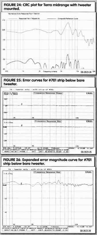 FIGURE 24: CRC plot for Terra midrange with tweeter mounted.
FIGURE 25: Error curves for #701 strip below bare tweeter.
FIGURE 26: Expanded error magnitude curve for #701 strip below bare tweeter.
I prepared strips of the three materials that were 6” long, 1” tall, and 1½” wide. With the 1½” face placed against the baffle, the strip nearly fills the gap between the midrange and tweeter and covers the full width of the two drivers. I performed the testing with the microphone back 1m. I replaced the midrange with a solid insert and installed the #701 strip below the tweeter. Figure 25 plots the error curves for the “ideal” tweeter when the #701 strip is installed. An expanded view of the error magnitude (Fig. 26) shows some small magnitude ripple. The CRC plot (Fig. 27) shows that the reflection from the #701 is down 20—30dB relative to the bare tweeter response and covers most of the frequency band.
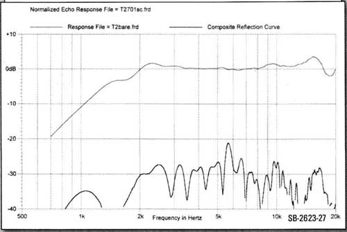
FIGURE 27: CRC plot for #701 strip below bare tweeter.

FIGURE 28: CRC plot for #703 strip below bare tweeter.
Figure 28 presents the CRC curve with the #703 strip installed. Compared to #701, the reflection starts to show the common bandpass shape. The low- and high-frequency levels are reduced, but the reflection level runs around -25dB from 2kHz to 7kHz.
Finally, Fig. 29 displays the CRC curve with the #705 strip installed. Compared to the #703 reflection, the high frequency is about the same, 2—7kHz a bit worse, and low frequencies improved. The #705 material seems great at absorbing lower frequencies, but shows a high reflection level in the midrange frequencies. When the damping strips are used with the mid range installed, it will be interesting to see whether the improvement in driver inter action is enough to offset the reflections from the strips themselves.

FIGURE 29: CRC plot for #705 strip below bare tweeter.
FIGURE 30: CRC plot for tweeter with midrange mounted—no strip.
FIGURE 31: Error curves for #701 strip between tweeter and midrange.

FIGURE 32: Expanded magnitude error curve for #701 strip between tweeter and
midrange.
FIGURE 33: CRC plot for #701 strip between tweeter and midrange.
FIGURE 34: CRC plot for #703 strip between tweeter and midrange.
DRIVER INTERACTION WITH STRIPS
I then installed the midrange in the test baffle with no damping strip. Because this was a new test setup, it was necessary to repeat the test of midrange interference on the tweeter’s response. The CRC curve for this setup is shown in Fig. 30. It shows the same bandpass shape as in Fig. 21 with the 3—5kHz wiggles replaced with a single dip. Figure 30 is the plot to which improvements made by the damping strips should be compared.
I installed the #701 strip (see the error curves in Fig. 31 and an expanded view of the magnitude errors in Fig. 32). The resulting CRC plot (Fig. 33) displays only modest improvement. The interference level is not improved in the 2—4kHz range, somewhat improved in the 4—8kHz range, and worse at high frequency due to the #701 strip’s own reflection. Because the tweeter would probably be used only above 3—4kHz, it appears the #701 strip would do more harm than good.
Figure 34 presents the CRC plot with the #703 strip installed. This strip shows some low-frequency improvement, but is worse above 5kHz where the tweeter would be used. The CRC plot with the #705 strip installed (Fig. 35) improves in the low—frequency area, but again is about the same or worse in the high- frequency range where the tweeter would be used.
In general the strips of high-density FG did not improve performance with a midrange driver mounted near the tweeter. Perhaps the felt used by Mr. Ralph and some varieties of foam materials would do better and should be tested. My past testing indicates felt is very good at high frequencies, while not very effective at low frequencies.
Part 2 will continue our look at interference problems affecting driver response.
REFERENCES
1. G.R. Koonce and R.O. Wright, “A Modest-Cost Three-Way Speaker System, Part 3,” Speaker Builder 8/96, p.3
2. G.R. Koonce with Kim Girardin, “Testing Front-Panel Damping Materials,” Speaker Builder 5/98, p. 32.
3. David B. Weems and G.R. Koonce, Great Sound Stereo Speaker Manual—Second Edition, McGraw-Hill, 2000, pp. 172—179.
4. David Ralph, “Diffraction Doesn’t Have to Be a Problem,” audioXpress June 2005, p. 55.
5. Jim Moriyasu, “A Study of Midrange Enclosures,” Speaker Builder 7/2000 and 8/2000.
6. Joe D’Appolito, “Testing the Parts Ex press MTM Kit,” audioXpress 4/05, Fig. 12, p. 61.

FIGURE 35: CRC plot for #705 strip between tweeter and midrange.
APPENDIX A:
HOW TO TEST FOR AND COMPUTE THE COMPOSITE REFLECTION CURVE DEVELOPING THE CRC MAGNITUDE CURVE
This work uses Liberty Instruments’ Audiosuite measurement system, but the approach should be applicable to any test set that allows you to define the curve used for calibration ( Cal). It is important to keep the test driver and microphone positions fixed throughout the test sequence. You must also keep the test signal level and all gains constant.
Remember that you will be performing computations on very small magnitude differences, so you need to maintain all the accuracy possible. I recommend using the MLS signal while averaging several tests. Also try to keep the noise in the test area to a minimum.
It is important for accurate results that you properly select the microphone distance and FFT window time. You need to make a valid far-field measurement, meaning the microphone should be back at least three times the maximum extent of the object under test. For multiple drivers the maximum extent is the largest of the total height, width, or diagonal of the multiple drivers; for a round GF it is the OD, and for rectangular GFs it is the outside diagonal. Also, the FFT window used must be long enough to include all the major ‘echoes” within the maximum extent of the test configuration and must be kept constant throughout the testing.
The first step is to test the bare driver (without the interfering object) in the normal way, allowing Audiosuite to generate a normal Cal correction. This produces the bare response for the driver under test to use as a reference. If you plan to compute the phase shift for the CRC plot, then the procedure from here on will change as discussed later. For CRC magnitude only computation, you would now export the bare driver response as an ASCII file.
You now again measure the bare driver response, but in single-channel mode with no calibrations. Save this curve and make it the special Cal curve for further testing. This curve contains the raw driver response along with any errors in the amplifier, wiring, and microphone and additionally contains the severe phase shift caused by the transit time from driver to microphone. When it is used as the Cal curve, it will subtract all these items from whatever you test next.
To verify the test approach is working properly, test the bare driver a third time using the special Cal curve just mentioned. This generates the error curve for no change in the test system. If everything is perfect, you are subtracting two identical curves, producing the results of straight lines at 0dB and zero degrees phase shift.

FIGURE 1A: Error curves for repeat test of bare Terra tweeter.
FIGURE 2A: Expanded plot of magnitude error in repeat test

FIGURE 3A: CRC plot for repeat test on bare Terra tweeter.
FIGURE 4A: Error curves for round OF with felt no time correction.
Figure 1A displays such results for the bare Terra tweeter. Figure 2A is an expanded view of the error magnitude which really moves about a fraction of a dB. The error curves were exported as an ASCII file and processed by the CRC program. Figure 3A gives the results indicating the test approach has a background interference level of -35dB or so. You need to have your procedure “clean” enough that you can produce this kind of background level.
At this point you make the change that represents the interference you choose to compare to the bare driver. Be careful not to move the test driver or the microphone. Now measure the response of the driver with interference using the special Cal curve.
Figure 4A shows the results when this was done for the round grille frame with four layers of fiberglass. The magnitude curve is fine but the phase shift curve has some error, as it should go to zero at high frequency. This error is due to something being physically moved or a change in the acoustic origin of the driver.
I found that interfering objects tend to slightly change the acoustic origin position, causing a phase error. You must use Audio- suite’s Compensate to insert a time correction to move the phase shift to zero at high frequency. The phase curve in Fig. 4A took a time correction of 9 to yield the phase curve back in Fig. 9 of the text.
The time corrections are usually small, but if you do not make them the CRC magnitude will show a rising amplitude at high frequency which is not valid. If you move the driver’s acoustic origin, such as by comparing a surface-mounted versus flush- mounted driver, the time correction will be much larger and it is critical that it be made. Once you have the error curves the way you want them, output them as an ASCII file.
While you could pick data out of the ASCII files to make the computations by hand at a few desired frequencies, the better approach is to write a short computer program to take in the ASCII files and then compute and plot the CRC magnitude curve. The program reads in the bare driver ASCII file and uses only the magnitude values, unless you choose to plot phase shift as covered later. The program reads the error curves ASCII file where it uses both the magnitude and phase shift information.
MAKING THE CALCULATION
The data shown in the error file is the vector sum of two items. The first is the “ideal” driver response at 0dB and zero degrees phase shift at all frequencies. This vector is thus always magnitude = 1, angle = 0. The second item is the CRC, which you want to recover. Thus the CRC is a vector equal to the error vector minus the “ideal” driver vector. At each frequency:
CRC vector = ((Em * Cos(Ep)) - 1) + j (Em * Sin(Ep)) in polar notation where Em is the error signal magnitude (as a number, not in dB), and Ep is the error signal phase (in the format your computer pro gram requires). The * symbol means “times.”
The real part of the CRC vector = Re = ((Em * Cos(Ep)) - 1)
The imaginary part is = Tm = (Em * Sin(Ep))
The CRC magnitude = CRC = J((Re * Re) + (Tm * Im))
The CRC magnitude in dB would be=20*Log(
Now this gives the value of the CRC normalized to the “ideal” driver response.
To re-normalize it to your actual driver, add the dB value of the bare driver response at each frequency. For a plot that is easy to understand, I generally move the bare driver response so that it sets on 0dB. You can do this by adding the needed constant dB value to both curves (bare driver and CRC) at each frequency
THE CRC PHASE SHIFT CURVE
The CRC phase shift curve is more difficult. The computation is not difficult, it is the re-normalization that causes the problem as you need the bare driver true phase shift data. The phase data normally exported with the bare driver ASCII file includes the phase shift caused by the sound transit time from the driver to the microphone. So for CRC phase shift plots, you must start right with the testing to obtain the proper bare driver phase shift curve.
There is a simple, but not always accurate, approach. Audiosuite will compute the Hilbert phase shift, which is the driver phase shift based on its frequency magnitude response assuming the driver is minimum- phase throughout the test range. So one approximate approach is to have your test set substitute the Hilbert phase shift for the bare driver response before you export the ASCII file.
The better approach is to try to establish the actual driver phase shift response by adding the right time compensation to remove the transit-time phase shift. This can become a bit of trial-and-error. Keep in mind that Audiosuite’s preamp contains a sometimes confusing phase inversion. I solve this by connecting the driver under test with inverted polarity.
After saving the measured bare driver response to a file, I have Audiosuite do the Hubert transform and print the response with magnitude and phase shift. This gives me an idea of what the phase should look like when I recall the original bare driver response and play with compensation times. Figure 5A shows the Hilbert phase shift for the Terra tweeter with the midrange present. Figure 6A shows the measured phase shift generated by adding the proper time compensation. The differences are slight except at the frequency extremes.

FIGURE 5A: Hubert Phase for Terra tweeter with mid range mounted.
Once you have exported the bare driver response with the proper phase shift, testing and computation, proceed as above for no phase shift curve. Once you compute the real (Re) and imaginary (Tm) values for the CRC vector you must then compute the phase shift.
CRC phase = Arctan(Im/Re)

FIGURE 6A: Measured phase for Terra tweeter with midrange mounted.
Make sure that you compute the phase in the proper quadrant. This gives you the phase shift for the CRC relative to the “ideal” driver. To re-normalize this to the actual driver, add these phase shift values to the bare driver-phase shift values. You could then plot the CRC phase shift relative to the source signal.
I did not believe that the phase shift curve added enough information to be worth the trouble. The magnitude of the CRC curve tells you how much trouble you are in. Phase shift determines direction—whether you get a response dip or peak—and weight of the CRC magnitude applied against the reference response. If you modify your construction so that the CRC magnitude is reduced sufficiently then you don’t care what the CRC phase shift is.
a: Most of you were probably expecting the term “acoustic center” for the location in space from which a driver appears to radiate. In a personal communication, GLA pointed out to me that because acoustic center had two definitions in the audio field, the preferred term for the driver radiation location is now “acoustic origin.”