The previous Section enabled us to bring a piece of audio equipment to a state where it could be used safely. In this final Section, we will assume that we have a working piece of equipment, but that we want to measure precisely how well it works - we might do this for a variety of reasons:
-- We hope to verify that it works as designed
-- We suspect that it can be improved, so we measure with a view to correction
-- We know that it works well and want some numbers to boast about.
Linear distortions
We should always measure linear distortion first because an unexpected result could force a minor circuit change affect non-linear distortion. By contrast, it is unusual for any change such as a bias adjustment required as a result of non-linear distortion to affect a linear distortion such as amplitude against frequency response.
Gain
The first measurement is likely to be a gain measurement. We apply a signal of known amplitude at the input of the amplifier and measure the amplitude at the output. The ratio of the two is the gain (G), also known as amplification (A):
Gain = Vout/Vin
The audio band is traditionally considered to range from 20Hz to 20 kHz, so to avoid errors caused by HF and LF roll-offs, gain is measured in the middle of this band using a sine wave having a frequency of 1 kHz.
If we apply too much signal to the amplifier, the signal at the output will be distorted, making the gain measurement inaccurate. To avoid distortion, and maximize accuracy, we apply a sufficiently small signal to the input of the amplifier to ensure that the output is undistorted. For this reason, gain is known as a small-signal measurement.
The whole point of making technical measurements is to provide a prediction of how well the equipment will work when used for its intended purpose, so our test level is important.
Professional audio equipment has tightly defined levels, but even domestic audio has reasonably well-defined levels. For example, the original CD standard defined that a CD player reproducing an undistorted sine wave at the maximum level permitted by the digital code (known as 0dBFS) should deliver an analog amplitude of 2VRMS. If a CD player is capable of delivering 2VRMS, it is not unreasonable to expect a pre-amplifier to be able to cope with this amplitude without distortion, so we could use this as our test level.
Although it is traditional to specify audio voltages in terms of VRMS, and meters are calibrated in terms of VRMS, gain does not change with amplitude, so there is no reason why we should not modify our test level slightly, to suit our particular test equipment ideally. Thus, if we were using an oscilloscope to measure gain, we would find it more convenient to use a sine wave having an amplitude of 6Vpk_pk (equivalent to 2.12VRMS) because this would occupy exactly six vertical divisions at 1V/div. (Although most oscilloscopes have eight vertical divisions, an analog display tube's linearity tends to deteriorate at extreme deflections.) It doesn't matter which form of measurement we use, just so long as we measure the input and output in the same way:
Vout / Vin = Vout [ pk-pk] / Vin [ pk-pk] = Gain
Dedicated audio test sets
Dedicated audio test sets invariably express their results in terms of decibels or dB:
Gain [dB] = 20 log [Vout [RMS] / Vin [RMS] ]
It's probably some time since you covered logarithms at school, so at the risk of offending those with better memories, the equation is used by first calculating the voltage ratio, then taking the common logarithm of the result (the ''log'' button on your calculator), and finally multiplying the result by twenty. Remember: Terms inside brackets first, then functions (logs, trig, etc.), then powers, then multiplication and division, and finally addition or subtraction.
One justification for this apparent complication is that if we have a chain of amplifiers with their gains specified in dB, we can find the total gain simply by adding all the gains (in dB) together. If we want to find the total gain when individual gains are expressed as ratios, we have to multiply all the gains together, which is somewhat harder.
Note that gain expressed in dB is still a ratio, albeit a logarithmic ratio. If we want to use dBs to express an absolute voltage, we must choose a reference voltage and compare our measured voltage to that reference. Many years ago, telecommunications companies sent analog audio over 600-ohm telephone lines, and in order to express levels in terms of dBs, they defined a reference level of 1mW dissipated in 600-ohm, and called this level 0dBm (m for milliwatt). Power is quite difficult to measure, so their meters actually measured the voltage across a 600-ohm resistor and the meter scales were calibrated in terms of the power dissipated in that resistor. Nobody uses 600-ohm any more, yet audio test sets are still saddled with this legacy, even though they usually measure the voltage across entirely different impedances. Because of this, the modern parlance is dBu, which corresponds to the same voltages as dBm, but ignores the 600-ohm impedance requirement.
We can find the voltage required to dissipate 1mW in 600-ohm by rearranging P=V2 /R to give:
V = 0.775VRMS
Because this voltage is derived from power, it must be specified in terms of VRMS, and this is why VRMS is popular for audio.
Now we know that 0.775VRMS would dissipate 1mW in 600-ohm, we can deem this to be our reference level, and call it 0 dBm if we truly are using 600-ohm impedances, or 0 dBu if we are ignoring impedances.
20VRMS in dBu:
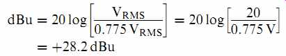
Note that when using dBu, it is conventional to state explicitly that the number is positive. Smaller voltages can easily produce negative values.
3.54mVRMS in dBu:
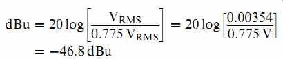
It is also conventional to specify AC measurements in dBs to only one decimal place unless you have stunningly accurate test equipment, because it is quite difficult to measure AC more accurately than 1%, and this corresponds to ~0.1 dB.
Conversely, you might have made a measurement in dBs but need to convert it back into a voltage ratio. In which case:
V1/V2 = 10 dB 20 [+ 16 dB expressed as a voltage ratio:
V1/ V2 = 10 dB 20 [+ = 10 16 20 [+ = 6:31
_16 dB expressed as a voltage ratio:
V1/V2 = 10 dB 20 [+ = 10
_16 20 [+ = 0:158
+16 dBu expressed as an absolute voltage:
VRMS = 0:775VRMS _ 10 dB 20 [+ = 0:775VRMS _ 10 16 20 [+
= 4:89VRMS
+16 dBu expressed as an absolute voltage:

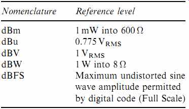
Note that the sign is absolutely critical, and that it is very important to be clear about whether you are using dB as a ratio or dBu as an absolute level. In addition to dBu, other audio references are in common use:
=======
============
Peak program meter scales
Peak program meter (PPM) scales were briefly mentioned in Section 4, but we now need to look at the scale and understand the logic behind it. The PPM was originated by the BBC for measuring the level of live program material and there were various requirements:
-- The program material would subsequently be presented to analog tape machines or transmitters employing amplitude modulation, neither of which forgive overload.
-- The meter would be read and interpreted by operators who were primarily concerned with making artistic adjustments to achieve the best sound balance.
-- The operators would be working under pressure, possibly with poor lighting.
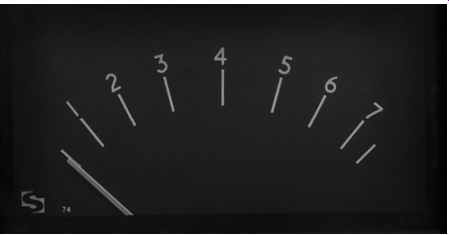
Fig. 1 The PPM scale is 4 dB/div, with 0 dBu = PPM4 (This is a stereo
PPM with a pair of back-to-back movements, hence the pair of pointers.)
Taken together, these requirements mean that the meter must be easy to read, and have a clear, uncluttered scale. An equal increment logarithmic scale of 4 dB/div means that meter deflection is proportional to loudness (see Fig.1).
White lettering on a black background makes the scale easy to read. 0 dBu=PPM4, and since there are 4 dB/div, PPM1=_12 dBu and PPM7= +12 dBu. Normal practice is to use 0 dBu as line-up level, and to mix program material so that peaks do not exceed PPM6, or +8 dBu. Although UK broadcasters use the 1-7 scale, European broadcasters mark the scale - 12 to +12. The meters are identical in all other respects [1].
When a PPM is used for engineering, all controls are referenced to PPM4. Thus, the level of the incoming signal can be read directly from the controls provided that they have been adjusted to set the PPM to read PPM4. PPMs intended for engineering use generally also include an expanded scale in addition to the PPM scale, and may include other scales, making them more cluttered, but they're not being used to mix live programs (see FIG. 2).
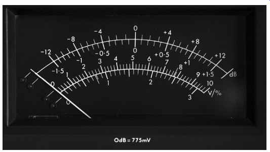
FIG. 2 Engineering PPMs always include an expanded scale in addition to
the PPM scale, and may include other scales
The unfortunate consequence of the 600W legacy
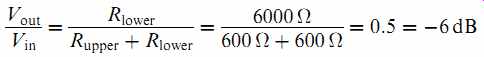
The reason that the telecommunications companies used 600-ohm is that their equipment drove cables that were so long that they really were transmission lines at audio frequencies. As an extreme example, there used to be a cable carrying program from Bush House in London to the transmitter at Daventry (67 miles away) without any intervening amplification. Because the cables were transmission lines, impedance matching was important, so the cables' characteristic impedance of 600-ohm had to be driven from a 600-ohm source and be terminated by a 600-ohm load. As a consequence, exchange (telecomms) and studio (broadcast) plant (electronic equipment) was all designed for 600-ohm impedance matching. The significance of this is that the input resistance of the destination formed a potential divider in conjunction with the source resistance driving it (see FIG. 3).
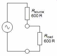
FIG. 3 The legacy of 600-ohm analog telecommunications is a 6 dB potential
divider to trap the unwary
Using the potential divider equation:
The modern technique is to make all devices have a high input impedance and a low output impedance. Thus:
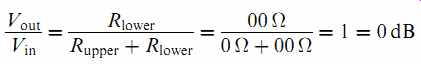
We can now see that the modern technique avoids a wasteful loss of 6 dB. The consequence is that if you set the attenuators on a 600-ohm audio oscillator to produce a specific output level, its output will be 6 dB high unless it is loaded or terminated by 600-ohm.Unless you know your oscillator, it is wisest to measure the signal at the input of the amplifier, rather than rely on the attenuators.
Source and load impedances for the Device Under Test (DUT) Having ensured that the oscillator is correctly terminated, we must also ensure that we terminate our DUT correctly.
If we are measuring a simple tube pre-amplifier, it might have an output impedance of ~6kOhm and expect to see a 1 M-ohm load.
A typical audio test set has an input impedance of 100 kOhm on its ''high'' setting, so this would cause an additional loss of 0.53 dB compared to a measurement with the correct 1 M-ohm loading.
Conversely, measuring with a 10:1 oscilloscope probe (10 M-ohm input resistance), would theoretically give a reading 0.054 dB high, but since this corresponds to +0.6%, it is comparable with oscilloscope error, so we would probably never notice it.
If we measure a power amplifier, we should terminate it with a load resistance appropriate to the secondary setting. Thus, if we have set the secondary to match a 4-Ohm load, we need a 4-ohm resistor, often known as a dummy load. Since we will almost certainly attempt to determine maximum output power, the resistor must be capable of withstanding this power without damage.
Unfortunately, wirewound resistors are not suitable as dummy loads because values <1kOhm have considerable inductance compared to their resistance. Fortunately, 50W non-inductive thick film resistors are available, and multiples of these can be screwed to a large heatsink to make a perfectly satisfactory dummy load (see FIG. 4).
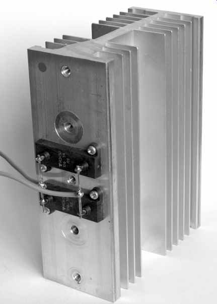
FIG. 4 A dummy load for testing power amplifiers can be made from thick-film
resistors screwed to a large heat sink
Whether the DUT is a power amplifier or a pre-amplifier, it should be driven from an appropriate source resistance.
Modern audio electronic equipment such as a CD player typically has an output resistance of _ 600-ohm. Some audio oscillators have selectable output resistance, whereas others are fixed, but the highest output resistance is generally 600-ohm, so any of these settings is appropriate. However, if you know that you will drive your DUT from a higher source resistance, perhaps from the output of a simple 100 kOhm logarithmic volume control, a 25kOhm series resistor should be added to emulate the maximum expected source resistance.
Measuring gain at different frequencies
Once we have taken the trouble to measure the gain correctly at 1 kHz, it is easy to leave all other controls alone, then change frequency, and take additional measurements to produce a graph of amplitude against frequency, which is habitually called ''frequency response''.
When we measured gain, it was equally valid to present the result as a pure voltage ratio (14) or in dBs (22.9 dB), but the purpose of measuring the amplitude against frequency response of an amplifier is to see if the amplitude deviates significantly from the 1 kHz level. This observation has two important implications:
-- Since we are worried about the audibility of amplitude deviations, we should use a logarithmic measurement because the ear/brain responds logarithmically. We should either measure directly in dBs or convert our measurement into dBs.
-- Absolute gain (or loss) is irrelevant, only deviations from the 1 kHz reference level matter. If we measured 1 kHz gain on a cathode follower pre-amplifier, we might have applied 0 dBu to the input of the DUT and measured ~0.6 dBu at the output. Rather than do lots of arithmetic, it is far easier to adjust the oscillator output level to produce precisely 0 dBu at 1 kHz at the output of the DUT, then (leaving oscillator level unchanged) measure output level at different frequencies and obtain the amplitude against frequency response directly.
Which frequencies to use? Because the ear/brain responds logarithmically, audio amplitude against frequency graphs are plotted on paper having a linear vertical scale (remember that dBs are already logarithmic) and a logarithmic horizontal scale. The most useful graph has equally spaced points, rather than a desert punctuated by oases of closely clustered points. Thus, we should choose measurement frequencies that produce equally spaced points on logarithmic paper.
We could use the oscilloscope attenuator logarithmic sequence of 1, 2, 5 to give equally spaced points, resulting in test frequencies of; 20Hz, 50Hz, 100Hz, 200Hz, 500Hz, 1 kHz, 2 kHz, 5 kHz, 10 kHz, and 20 kHz. Unfortunately, the points are rather sparse, so a better choice is to use International Standards Organization (ISO) recommendation 2661 3 octave frequencies:
20Hz, 25Hz, 31.5Hz, 40Hz, 50Hz, 63Hz, 80Hz, 100Hz, 125Hz, 160Hz, 200Hz, 250Hz, 315Hz, 400Hz, 500Hz, 1 kHz, 1.25 kHz, 1.6 kHz, 2 kHz, 2.5 kHz, 3.15 kHz, 4 kHz, 5 kHz, 6.3 kHz, 8 kHz, 10 kHz, 12.5 kHz, 16 kHz, 20 kHz.
Twenty-nine points are thus needed to cover the range from 20Hz to 20 kHz, and these frequencies would be entirely appropriate if we were measuring an RIAA pre-amplifier because their errors are perfectly capable of producing deviations at almost any point across the audio band. (Incidentally, fuse values follow the same logarithmic sequence; 2A, 2.5A, 3.15A, etc.) However, if we were measuring a typical power amplifier, this would be a wasted effort because it has a low frequency roll-off, a high frequency roll-off, and is flat in between (see FIG. 5). ISO 1 3 octave frequencies (and their multiples beyond 20 kHz) were used, resulting in a graph with evenly spaced points. As can be seen, the amplitude response against frequency is very nearly flat, and taking the measurements was tedious. When measuring a tube power amplifier, it is better to sweep low frequencies slowly up to 50Hz, to find any low-frequency bumps, then sweep from 10 to 500 kHz to spot undamped HF resonances due to the output transformer, and if no unpleasant resonances are found, simply determine the LF and HF frequencies for which the response is either 1 dB or 3 dB down compared to the 1 kHz reference level.
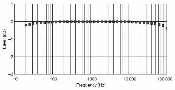
FIG. 5 Crystal Palace amplifier amplitude against frequency response taken
at an output power of 1W.
An even faster method than sweeping is to apply a 1 kHz square wave and check for negligible ringing at the leading edge, then apply a 100Hz square wave and select DC coupling at the input of the oscilloscope before checking that the top and bottom horizontal lines are truly horizontal, rather than sagging (sag indicates LF loss). Assuming that the square wave response is satisfactory, the _3 dB points can be determined using sine waves. If it isn't, there's not a lot of point in plotting a pretty graph of a HF or LF aberration, the problem needs to be corrected!
Plotting the graph
Having recorded our results neatly, we now need to plot them.
Considering the horizontal scale first, logarithmic graph paper is specified in terms of cycles and starts at 1. Thus, three-cycle logarithmic paper can cover 10Hz to 10 kHz, but we want to start at 20Hz and finish at 20 kHz, necessitating four cycle paper.
The vertical scale needs to be linear, and typical paper has minor divisions every millimeter and major divisions every centimeter. You were probably taught at school to choose a graph scale that used all of the graph paper, so you might find that a total range of +-2 dB to be sufficient to encompass your measurements. On typical paper, this approach would give a scale of 0.25 dB/cm, yet the measurement is probably only accurate to +-0.1 dB, so the very large graph would imply false accuracy. Worse, it could make a perfectly reasonable response look poor - an audibly flat response ought to look flat on paper. A sensible vertical scale is 2 dB/cm on typical office paper. This scale produces a graph that correlates well to the audible effects and does not display false accuracy.
Lin/log paper is expensive, and paper ideally suited to audio is unobtainable, so the author generated his own graph paper using a CAD package (see FIG. 6).
Measuring RIAA equalization using an inverse RIAA network
It is difficult to make a practical RIAA stage having perfect equalization because tubes vary from sample to sample and their characteristics change as they wear. It is therefore useful to have an inverse RIAA network that can be connected between an oscillator and the input of an RIAA stage so that the combination theoretically yields a flat amplitude response against frequency. If the inverse RIAA network is perfect, any deviation from flatness is due to the RIAA stage, so adjustments can be made until flatness is achieved.
Unfortunately, designing a ''perfect'' inverse RIAA network is not trivial. Factors that must be taken into account are:
-- The network is sensitive to source and load resistances, so it needs to be matchable to common oscillator output resistances.
-- The output resistance of the network should be similar to that of a typical cartridge, so that the (perhaps varying?) input impedance of the RIAA stage loads it correctly.
-- Unfortunately, the typical technique of designing an ideal RIAA equalizing circuit, preceding it with the inverse RIAA, and emulating it in an electronic analysis package tends to generate calculation errors. This is because the network analysis equations that can cope with general problems are more complex and more numerous than the optimized equations for a specific problem.
-- Capacitors are typically only available in 1%, but resistors are available in 0.1%, so errors should be limited to the capacitors. Further, it would be convenient if standard capacitor values could be used.
With these considerations in mind, the author started with the fundamental RIAA equation, and added the 3.18 ms time constant that has to be implemented at the time of cutting to protect the (probably Neumann) cutting head. The RIAA replay equation is therefore:
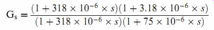
Where s=jω, and ω=2πf.
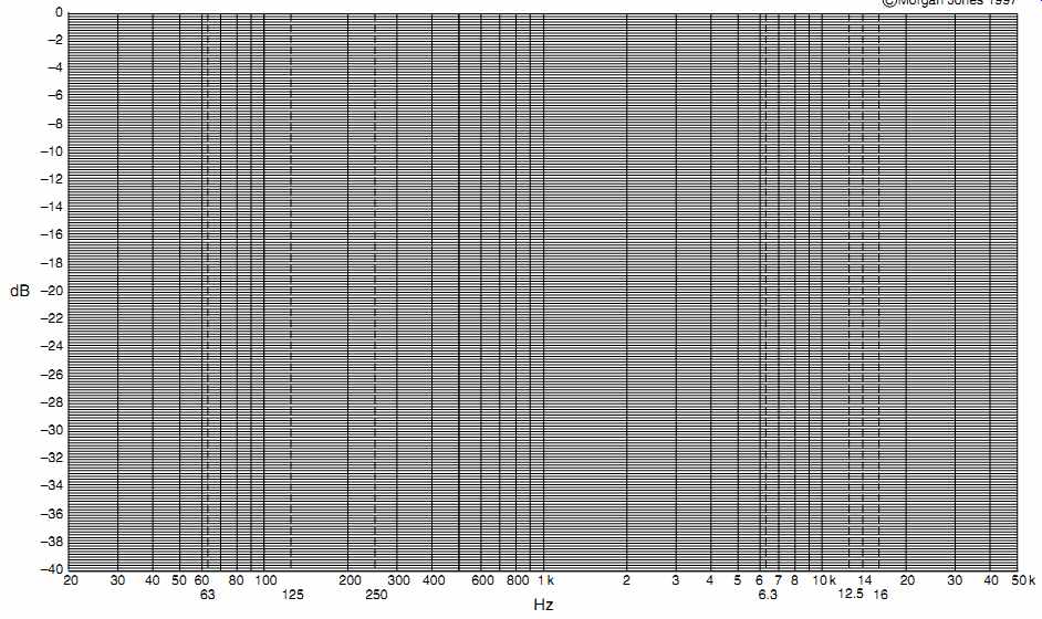
FIG. 6 Lin-log graph paper is difficult to obtain, so photocopy this ''audio''
paper.
Rather than re-invent the wheel, an existing inverse RIAA network developed by Jim Hagerman [2] from Stanley Lipshitz's [3] seminal AES paper was investigated, and the equation for its attenuation was written from first principles and entered into a spreadsheet. The fundamental RIAA replay equation was also entered into the spreadsheet, enabling the two equations to be multiplied together to generate a graph which should ideally show zero error (see FIG. 7).
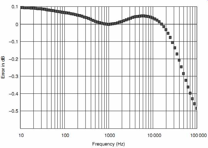
FIG. 7 The error curve for this commercial RIAA inverse network is quite
respectable despite being restricted to E24 component values.
Despite being restricted by E24 component values, the response is surprisingly good over the audio band. Nevertheless, every BBC audio test set from the ( tube) ATM/1 onwards is capable of measuring to better than 0.1 dB, so it seems worthwhile to improve matters.
The error worsens towards 100 kHz because the original Hagerman article used 3.5 ms, rather than 3.18ms. Although the less popular Ortofon cutting heads used 3.5ms rather the Neumann's 3.18ms, it is the author's experience that it is always preferable to use too little equalization than too much. Changing component values to set 3.18 ms, and making the fine adjustments possible by choosing 0.1% tolerance resistors available in E96 values significantly improves the design errors (see FIG. 8).
The design errors using single E24 capacitors and combinations of E96 and E24 resistors are now comfortably within +-0.01 dB, so the effect of practical components can be investigated. Since the capacitors are only available in 1% tolerance, the worst possible combination of capacitor tolerance extremes was investigated (see FIG. 9).
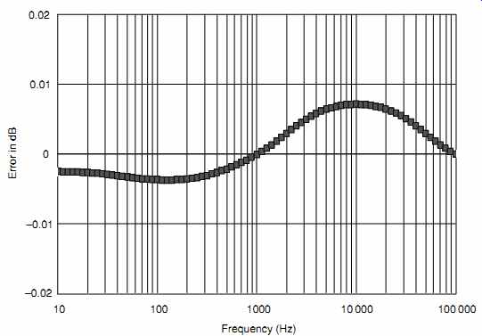
FIG. 8 Using a mix of E96 and E24 resistor values allows the design error
to be reduced greatly
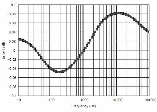
FIG. 9 The worst possible combination of capacitors errors produces this
frequency response error.
Even the worst possible combination of 1% capacitor tolerances leaves the predicted error better than +-0.1 dB. Because even a cheap function generator intrinsically has superb range flatness and constant output resistance with frequency, net work values were optimized to suit the output resistance of a typical function generator (see FIG. 10a).
Whether your function generator has an output resistance of 50 Ohm or 75 Ohm will determine whether you need a 47 Ohm or 22-ohm resistor respectively. The further advantage of matching the network to a function generator is that it allows square wave testing at the flick of a switch.
If the wires between the output of the oscillator and the network are more than a few inches long, and the function generator is flat to 10MHz, transmission line effects cause an overshoot on the leading edge of the square wave that can be misleading. If a longer cable cannot be avoided, use 50 Ohm co-axial cable, and modify the input of the network so that it (almost) correctly terminates the cable (see FIG. 10b).
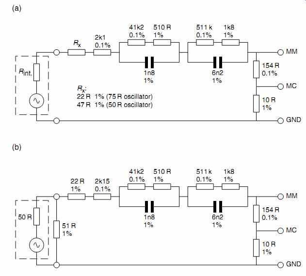
FIG. 10 Final circuit of inverse RIAA network.
This modification eliminates the overshoot at the expense of adding a slight tilt at the leading edge of a 10 kHz square wave.
Normal audio leads can be used to connect the output of either version to the pre-amplifier under test.