Types of code errors
When digital signals are sent through a transmission channel, or recorded and subsequently played back, many types of code errors can occur. Now, in the digital field, even small errors can cause disastrous audible effects: even one incorrectly detected bit of a data word will create an audible error if it is, say, the MSB of the word.
Such results are entirely unacceptable in the high quality expected from digital audio, and much effort must be made to detect, and subsequently correct, as many errors as possible without making the circuit over-complicated or the recorded bandwidth too high.
There are a number of causes of code errors:
Dropouts
Dropouts are caused by dust or scratches on the magnetic tape or CD surface, or microscopic bubbles in the disc coating.
Tape dropout causes relatively long-time errors, called bursts, in which long sequences of related data are lost together. On discs dropouts may cause either burst or single random errors.
Jitter
Tape jitter causes random errors in the timing of detected bits and, to some extent, is unavoidable, due to properties of the tape transportation mechanism. Jitter margin is the maximum amount of jitter which permits correct detection of data. If the minimum run length of the signal is t, then the jitter margin will be t/2.
FIG. 1 shows this with an NRZ signal.
Intersymbol interference
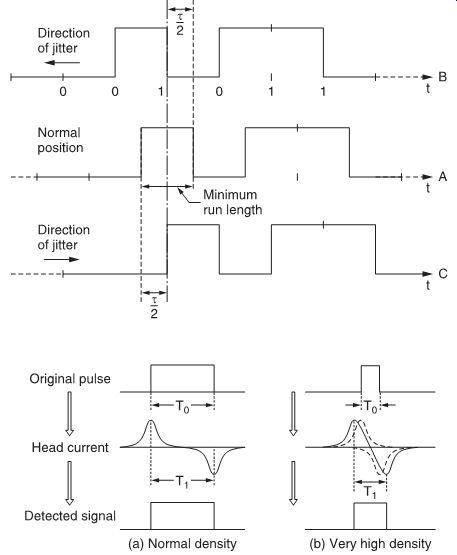
FIG. 1 Jitter margin.
FIG. 2 The cause of intersymbol interference.
In stationary-head recording techniques, a pulse is recorded as a positive current followed by a negative current (see FIG. 2).
This causes the actual period of the signal that is read on the tape (T1 ) to be longer than the bit period itself (T0 ). Consequently, if the bit rate is very high, the detected pulse will be wider than the original pulse. Interference, known as intersymbol interference or time crosstalk, may occur between adjacent bits.
Intersymbol interference causes random errors, depending upon the bit situation.
Noise
Noise may have similar effects to dropouts (differentiation between both is often difficult), but random errors may also occur in the case of pulse noise.
Editing
Tape editing always destroys some information on the tape, which consequently must be corrected. Electronic editing can keep errors to a minimum, but tape-cut editing will always cause very long and serious errors.
Error compensation
Errors must be detected by some error-detection mechanism: if misdetection occurs, the result is audible disturbance. After detection, an error-correction circuit attempts to recover the correct data. If this fails, an error-concealment mechanism will cover up the faulty information so, at least, there is no audible disturbance.
These three basic functions--detection, correction and concealment--are illustrated in FIG. 3.
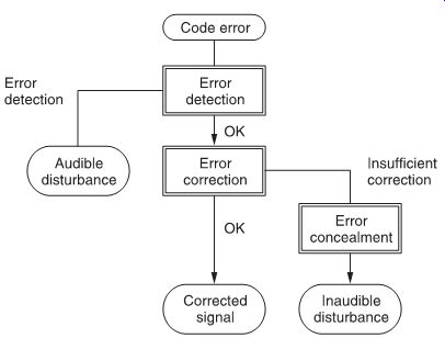
FIG. 3 Three basic functions of error compensation: detection, correction
and concealment.
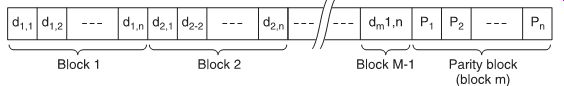
FIG. 4 Extended parity checking.
Error detection
Simple parity checking--To detect whether a detected data word contains an error, a very simple way is to add one extra bit to it before transmission. The extra bit is given the value 0 or 1, depending upon the number of ones in the word itself. Two systems are possible: odd parity and even parity checking.
• Odd parity: where the total number of ones is odd.
Example:
1110 0 data parity 1001 1 data parity
• Even parity: where the total number of ones is even.
Example:
1110 1 data parity 1001 0 data parity
The detected word must also have the required number of ones.
If this is not the case, there has been a transmission error.
This rather elementary system has two main disadvantages:
1 Even if an error is detected, there is no way of knowing which bit was faulty.
2 If two bits of the same word are faulty, the errors compensate each other and no errors are detected.
Extended parity checking
To increase the probability of detecting errors, we can add more than one parity bit to each block of data. FIG. 4 shows a system of extended parity, in which M-1 blocks of data, each of n bits, are followed by block m--the parity block. Each bit in the parity block corresponds to the relevant bits in each data block, and follows the odd or even parity rules outlined previously.
If the number of parity bits is n, it can be shown that (for reasonably high values of n) the probability of detecting errors is 1/2 n.
Cyclic redundancy check code (CRCC)
The most efficient error-detection coding system used in digital audio is cyclic redundancy check code (CRCC), which relies on the fact that a bit stream of n bits can be considered an algebraic polynomial in a variable x with n terms. For example, the word 10011011 may be written as follows:
M(x) = 1x7
+ 0x6
+ 0x5
+ 1x4
+ 1x3
+ 0x2
+ 1x1
+ 1x0
= x7
+ x4
+ x3
+ x + 1
Now to compute the cyclic check on M(x), another polynomial G(x) is chosen.
Then, in the CRCC encoder, M(x) and G(x) are divided:
M(x)/G(x) = Q(x) + R(x) where Q(x) is the quotient of the division and R(x) is the remainder.
Then (FIG. 5), a new message U(x) is generated as follows:
U(x) = M(x) + R(x) so that U(x) can always be divided by G(x) to produce a quotient with no remainder.
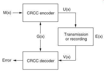
FIG. 5 CRCC checking principle.
It is this message U(x) that is recorded or transmitted. If, on play back or at the receiving end, an error E(x) occurs, the message V(x) is detected instead of U(x), where:
V(x) = U(x) + E(x)
In the CRCC decoder, V(x) is divided by G(x), and the resultant remainder E(x) shows there has been an error.
Example (illustrated in FIG. 6):
the message is M(x) = x9
+ x5
+ x2
+ 1 the check polynomial is G(x) = x5
+ x4
+ x2
+ 1
Now, before dividing by G(x), we multiply M(x) by x5; or, in other words, we shift M(x) five places to the left, in preparation of the five check bits that will be added to the message:
x5 M(x) = x14
+ x10
+ x7
+ x5 Then the division is made:
So that:
U(x) = x5 M(x) + (x + 1)
=x14
+ x10
+ x7
+ x5
+ x + 1 which can be divided by G(x) to leave no remainder.
FIG. 6 shows that, in fact, the original data are unmodified (only shifted), and that the check bits follow at the end.
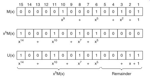
FIG. 6 Generation of a transmission polynomial.
CRCC checking is very effective in detection of transmission error. If the number of CRCC bits is n, detection probability is 1--2-n. If, say, n is 16, as in the case of the Sony PCM-1600, detection probability is 1--2-16
= 0.999985 or 99.9985%. This means that the CRCC features almost perfect detection capability. Only if E(x), by coincidence, is exactly divisible by G(x) will no error xMx Gx xxxxxx x 5 98732 1 1 ()/ () ()
=
+ ()
+
+ quotient remainder
be detected. This obviously occurs only rarely and, knowing the characteristics of the transmission (or storage) medium, the polynomial G(x) can be chosen such that the possibility is further minimized.
Although CRCC error checking seems rather complex, the divisions can be done relatively simply using modulo-2 arithmetic.
In practical systems LSIs are used which perform the CRCC operations reliably and fast.
Error correction
In order to ensure later correction of binary data, the input signal must be encoded by some encoding scheme. The data sequence is divided into message blocks, then each message block is transformed into a longer one, by adding additional information, in a process called redundancy.
The ratio (data + redundant data)/data is known as the code rate.
There is a general theory, called the coding theorem, which states that the probability of decoding an error can be made as small as possible by increasing the code length and keeping the code rate less than the channel capacity.
When errors are to be corrected, we must not only know that an error has occurred, but also exactly which bit or bits are wrong.
As there are only two possible bit states (0 or 1), correction is then just a matter of reversing the state of the erroneous bits.
Basically, correction (and detection) of code errors can be achieved by adding to the data bits an additional number of redundant check bits. This redundant information has a certain connection with the actual data, so that, when errors occur, the data can be reconstructed again. The redundant information is known as the error-correction code. As a simple example, all data could be transmitted twice, which would give a redundancy of 100%. By comparing both versions, or by CRCC, errors could easily be detected, and if some word were erroneous, its counter part could be used to give the correct data. It is even possible to record everything three times; this would be even more secure.
These are, however, rather wasteful systems, and much more efficient error-correction systems can be constructed.
The development of strong and efficient error-correction codes has been one of the key research points of digital audio technology. A wealth of experience has been used from computer technology, where the correction of code errors is equally important, and where much research has been carried out in order to optimize correction capabilities of error-correction codes.
Design of strong codes is a very complex matter, however, which requires thorough study and use of higher mathematics: algebraic structure has been the basis of the most important codes. Some codes are very strong against 'burst' errors, i.e., when entire clusters of bits are erroneous together (such as during tape dropouts), whereas others are better against 'random' errors, i.e., when single bits are faulty.
Error-correction codes are of two forms, in which:
1 Data bits and error-correction bits are arranged in separate blocks; these are called block codes. Redundancy that follows a data block is only generated by the data in that particular block.
2 Data and error correction are mixed in one continuous data stream; these are called convolutional codes. Redundancy within a certain time unit depends not only upon the data in that same time unit, but also upon data occurring a certain time before. They are more complicated than, and often superior in performance to, block codes.
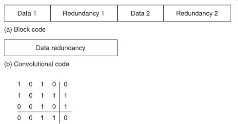
FIG. 7 Main differences between block and convolutional error-correcting
codes.

FIG. 8 Combinational parity checking.
FIG. 7 illustrates the main differences between block and convolutional error-correcting codes.
Combinational (horizontal/vertical) parity checking
If, for example, we consider a binary word or message consisting of 12 bits, these bits could be arranged in a 3 × 4 matrix, as shown in FIG. 8.
Then, to each row and column one more bit can be added to make parity for that row or column even (or odd). Then, in the lower right-hand corner, a final bit can be added that will give the last column an even parity as well; because of this the last row will also have even parity.
If this entire array is transmitted in sequence (row by row, or column by column), and if during transmission an error occurs to one bit, a parity check on one row and on one column will fail; the error will be found at the intersection and, consequently, it can be corrected. The entire array of 20 bits, of which 12 are data bits, forms a code word, which is referred to as a (20, 12) code. There are 20--12 = 8 redundant digits.
All error-correcting codes are more or less based on this idea, although better codes, i.e., codes using fewer redundant bits than the one given in our example, can be constructed.
Crossword code Correction of errors to single bits is just one aspect of error correcting codes. In digital recording, very often errors come in bursts, with complete clusters of faulty bits. It will be obvious that, in view of the many possible combinations, the correction of such bursts or errors is very complicated and demands powerful error-correcting codes.
One such code, developed by Sony for use in its PCM-1600 series, is the crossword code. This uses a matrix scheme similar to the previous example, but it carries out its operations with whole words instead of individual bits, with the resultant advantage that large block code constructions can be easily realized so that burst error correction is very good. Random error correction, too, is good. Basically, the code allows detection and correction of all types of errors with a high probability of occurrence, and that only errors with a low probability of occurrence may pass undetected.
A simple illustration of a crossword code is given in FIG. 9, where the decimal numbers represent binary values or words.
FIG. 10 shows another simple example of the crossword code, in binary form, in which four words M1
-M4 are complemented in the coder by four parity or information words R5
-R8 , so that:
where the symbol ? denotes modulo-2 addition.
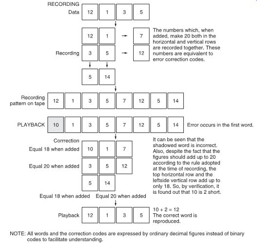
FIG. 9 Illustration of a crossword code.
All eight words are then recorded, and at playback received as U1-U8.
In the decoder, additional words are constructed, called syndrome words, as follows:
SUU U SUUU SUUU SUUU 11 2 5 2346 3137 4248
=??
=??
=??
=??
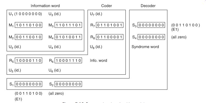
FIG. 10 Crossword code using binary data.
By virtue of this procedure, if all received words U1 -U8 are correct, all syndromes must be zero. On the other hand, if an error E occurs in one or more words, we can say that:
Now:
as we know that M1
? M2
? R5
= 0. Similarly:
Correction can then be made, because:
Of course, there is still a possibility that simultaneous errors in all words compensate each other to give the same syndrome patterns as in our example. The probability of this occurring, however, is extremely low and can be disregarded.
SUU U MEMERE EEE 11 2 5 11 22 55 125
=??
=?????
=?? SEEE SEEE SEEE 2346 3137 4248
=??
=??
=?? USMEEM 13 111 1 ?= ??=
Ui
= Mi
? Ei for i = 1-4 Ui
= Ri
? Ei for i = 5-8
In practical decoders, when errors occur, the syndromes are investigated and a decision is made whether there is a good probability of successful correction. If the answer is yes, correction is carried out; if the answer is no, a concealment method is used.
The algorithm the decision-making process follows must be initially decided using probability calculations, but once it is fixed it can easily be implemented, for instance, in a P-ROM.
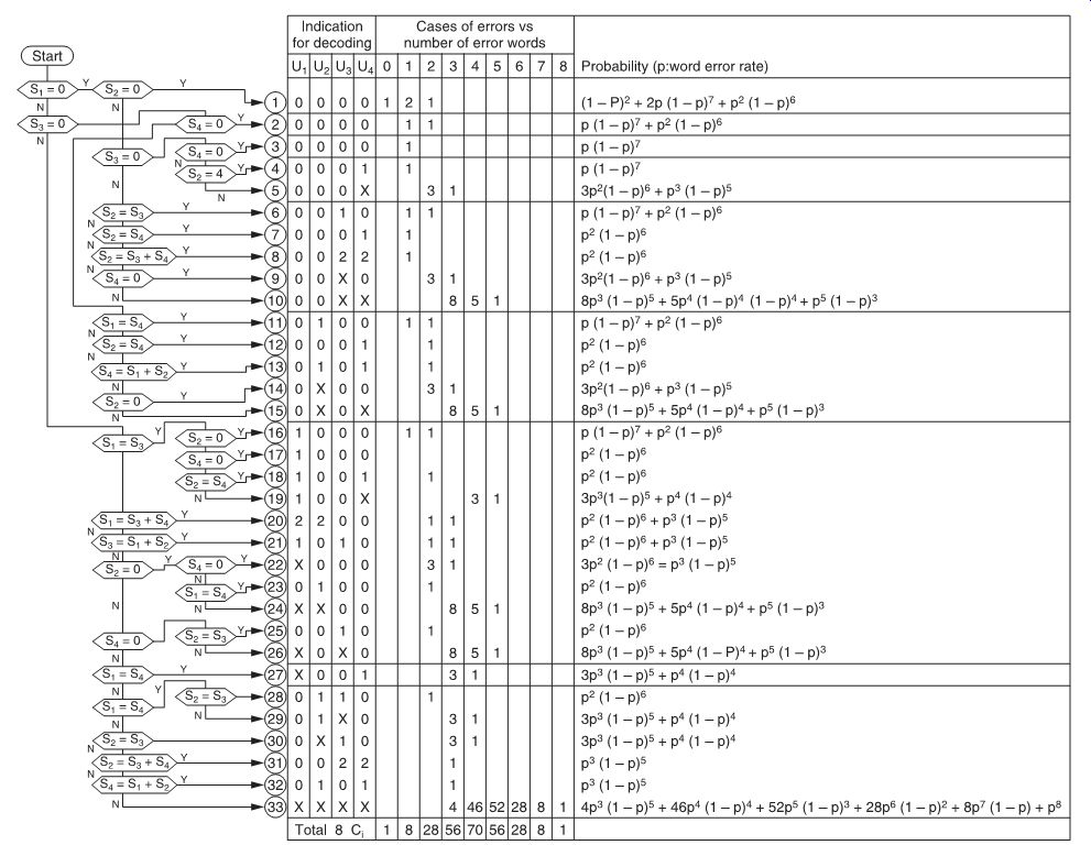
FIG. 11 Decoding algorithm for crossword code.
FIG. 11 shows the decoding algorithm for this example crossword code. Depending upon the value of the syndrome(s), decisions are made for correction according to the probability of miscorrection; the right column shows the probability of each situation occurring.
b-Adjacent code
A code which is very useful for correcting both random and burst errors has been described by D. C. Bossen of IBM, and called b adjacent code. The b-adjacent error-correction system is used in the EIAJ format for home-use helical-scan digital audio recorders.
In this format two parity words, called P and Q, are constructed as follows:
where T is a specific matrix of 14 words of 14 bits; Ln, Rn, etc. are data words from, respectively, the left and the right channel.
CIRC code and other codes Many other error-correcting codes exist, as most manufacturers of professional audio equipment design their own preferred error-correction system.
Most, however, are variations on the best-known codes, with names such as Reed-Solomon code and BCH (Bose-Chaudhuri- Hocquenghem) code, after the researchers who invented them.
Sony (together with Philips) developed the cross-interleave Reed-Solomon code (CIRC) for the compact disc system. R-DAT tape format uses a double Reed-Solomon code, for extremely high detection and correction capability. The DASH format for professional stationary-head recorders uses a powerful combi nation of correction strategies, to allow for quick in/out and editing (both electric and tape splice).
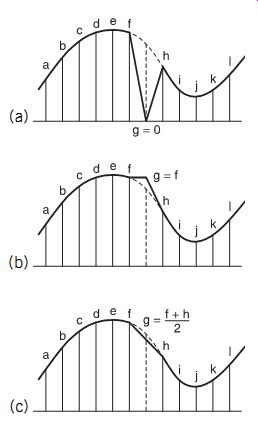
FIG. 12 Three types of error concealment: (a) muting; (b) previous word
holding; (c) linear interpolation.
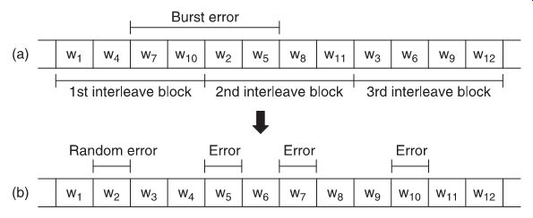
FIG. 13 How interleaving of data effectively changes burst errors into
random errors.
Error concealment
Next comes a technique which prevents the uncorrected code errors from affecting the quality of the reproduced sound. This is known as concealment, and there are four typical methods.
1 Muting: the erroneous word is muted, i.e., set to zero (FIG. 12a). This is a rather rough concealment method, and consequently used rarely.
2 Previous word holding: the value of the word before the erroneous word is used instead (FIG. 12b), so that there is usually no audible difference. However, especially at high frequencies, where sampling frequency is only two or three times the signal frequency, this method may give unsatisfactory results.
3 Linear interpolation (also called averaging): the erroneous word is replaced by the average value of the preceding and succeeding words (FIG. 12c). This method gives much better results than the two previous methods.
4 Higher-order polynomial interpolation: gives an estimation of the correct value of the erroneous word by taking into account a number of preceding and following words.
Although much more complicated than the previous methods, it may be worthwhile using it in very critical applications.
Interleaving
In view of the high recording density used to record digital audio on magnetic tape, dropouts could destroy many words simultaneously, as a burst error. Error correction that could cope with such a situation would be prohibitively complicated and, if it failed, concealment would not be possible as methods like interpolation demand that only one sample of a series is wrong.
For this reason, adjacent words from the A/D converter are not written next to each other on the tape, but at locations a sufficient distance apart to make sure that they cannot suffer from the same dropout. In effect, this method converts possible long burst errors into a series of random errors. FIG. 13 illustrates this in a simplified example. Words are arranged in interleave blocks, which must be at least as long as the maximum burst error. Practical interleaving methods are much more complicated than this example, however.