
VECTORS
A vector is a means of graphically representing any quantity that has both magnitude and direction. It is a shorthand method of illustrating a problem without the use of algebra. Vectors are used a great deal in electrical work where a-c quantities become complex when represented mathematically. Complex mathematics are, thus, avoided by the use of vectors which graphically represent desired relation ships. In this text vectors are used specifically to represent the magnitude and phase relationships of a-c quantities.
A vector is usually depicted by an arrow, with the arrowhead indicating the direction of the quantity. The direction of a vector quantity is measured in degrees, these degrees being based upon the 360 degrees in a circle. The vectors in this guide are drawn with respect to a coordinate system, as shown in Fig. A-1. It should be remembered, even when these reference axes are omitted, that vector representation is based upon such a system.
Counterclockwise rotation of the vector from the reference axis is considered positive, and clockwise rotation of the vector is considered negative. If one vector is drawn ahead of another in the counter clockwise direction, the former vector is said to be leading the latter by so many degrees phase difference (phase angle). For instance, in Fig. A-1 vector B is leading vector A by 45°, since 45° is the difference
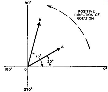
Fig. A-1. As rotation in the counterclockwise direction is considered
positive, vector B leads vector A by 45 °, the difference between the
angular displacements of 30° and 75°. Vector A may also be considered
to lag vector B by 45 °; the two vectors are also said to be out of phase
by 45°.
in their angular displacements from zero. Another way of stating this relationship is to say that vector A is lagging vector B by 45°. Two different vectors are illustrated in Fig. A-1, although any number of vectors can be drawn on the same set of axes. Vector A ( or vector OA as it is often called) represents a quantity that has a phase angle of 30°, and vector B represents a quantity that has a phase angle of 75°. The phase difference between these two angles is 45 °. Vectors A and B can represent current, voltage, or impedance. They need not represent the same kind of quantities, even though they are drawn with respect to the same set of axes.
Vectors are used to portray different things such as phase and magnitude relationships, algebraic operations (addition, subtraction, and so forth) and the component parts of a-c quantities. In Fig. A-1, the phase relationship between the two vectors A and B is illustrated.
It should be remembered that all vector operations are algebraic in nature and involve something more than simple arithmetical calculations. The only vector operation that is used throughout this guide is vector addition. When vectors are added the resultant vector is not necessarily greater than the individual vectors; the phase of the vector quantities is the factor which determines the magnitude of the resultant.
In vector addition only those vectors representing the same type of quantities can be added. That is, a voltage vector can be added to another voltage vector, but not to a current or impedance vector. Similarly, a current vector can be added only to some other current vector and not to a voltage or impedance vector. The simplest type of vector addition is that between two in-phase or 180° out-of-phase vectors.
When adding in-phase vectors, the magnitude (or length) of one vector is added arithmetically to the other. When vectors are 180° out of phase, the algebraic addition involves the arithmetical subtraction of the magnitude (or length) of the smaller vector from the larger to get the resultant vector.
Vector addition involving phase differences of other than 180° is carried out in a different manner. There are three principal methods used for adding vectors, the parallelogram method, the head-to-tail method, and the resolution method. The parallelogram method is used exclusively in this guide, so it is the only method discussed here. For a more comprehensive study of vectors, including all types of addition, other vector operations, and also their application to typical radio problems, see the guide "Understanding Vectors and Phase" by the authors of this text.
Addition by the Parallelogram Method
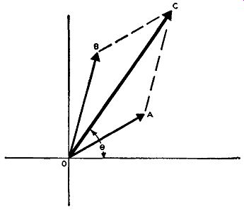
Fig. A-2. In order to add vectors A and B, the lines AC and BC are drawn
parallel to OB and OA respectively from the ends of the vectors A and
B. The diagonal OC of the resulting parallelogram is the vector sum of
the two vectors A and B, and has a phase angle theta.
When vectors are added by this method, the two vectors involved are used as the adjacent sides of a parallelogram. A parallelogram is a four sided figure, wherein the opposite sides are equal and parallel to each other. The lines connecting the opposite corners of a parallelogram are known as the diagonals. The vector addition is done by completing the parallelogram, and the diagonal connecting the angle formed by the adjacent vectors to the angle opposite it, is called the resultant vector.
In Fig. A-2, you will notice that vectors A and B of Fig. A-1 have been here added by the parallelogram method. Vectors A and B were used as the adjacent sides of a parallelogram, and the parallelogram OACB completed. In this drawing side BC is equal and parallel to side OA, and side AC is equal and parallel to side OB. A diagonal is then drawn from point theta (the origin of the coordinate system) to the opposite corner of the parallelogram. This diagonal, designated as line OC in Fig. A-2, is the resultant vector of the addition of vectors A and B and it has a phase angle of theta. Resolution of a Vector As was previously mentioned, a-c quantities are complex and to express them mathematically requires the use of complex algebra.
All a-c quantities, whether voltage, current, or impedance, may contain both resistive and reactive components. This is widely known to exist for impedance and it must, therefore, also hold for current and voltage. For instance, if an alternating current is said to have a magnitude of 10 amperes and a phase angle of 60°, it means that the current is composed of a resistive current of 5 amperes and a reactive current of 8.66 amperes.
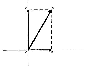
Fig. A-3. When revolving vector OD, line DF is drawn perpendicularly
to the horizontal axis at F and line DE is drawn perpendicularly to the
vertical axis at E. Lines OF and OE are the resulting horizontal and
vertical components respectively.
The resistive and reactive components of voltage, current, or impedance vectors can be simply found by resolving the vector. This is illustrated in Fig. A-3, where vector D can represent either a voltage, current, or series impedance. To resolve this vector into its component parts, we draw a rectangle using line OD as a diagonal of this rectangle. In this rectangle line DF is equal and parallel to line OE, and line ED is equal and parallel to line OF. The vertical line dropping from D is-perpendicular to the abscissa (horizontal axis) at F and the horizontal line leading from D is perpendicular to the ordinate (vertical axis) at E. The lines OF and OE are the horizontal and vertical components, respectively, of vector D. Horizontal component OF is the resistive part of vector D and vertical component OE is the re-active part. Vertical component OE indicates that the reactive part is inductive, for it lies on the upper or positive half of the ordinate axis.
If the reactance were capacitive, the vector would have appeared in the fourth quadrant, and the vertical component would fall on the bottom or negative half of the ordinate axis.
POWERS OF TEN
Powers of ten are a shorthand method of representing a large or a small number. It is especially useful in electrical work where such quantities as micromicrofarads, megohms, megacycles can be abbreviated mathematically.
In order to multiply a number by itself we write X2 where X is the number and the small number 2 means that X is to be multiplied by itself two times and is commonly referred to as X squared. If 2 were replaced by a 3 or 4 or any other number we would have X3 or X4, and so on. The 3 means that X is multiplied by itself 3 times, and the 4 means that X is multiplied by itself 4 times and so on. These numbers 2, 3, 4, and so on, are called exponents or power numbers. Thus X2, usually called X squared, can also be called X raised to the second power. Therefore, X3 means X to the third power and X4 means X to the fourth power. By such statements we readily associate the power form or exponent as meaning the number of times X is multiplied by itself.
Consequently, the number 10^2 means 10 X 10 or 100; 10^3 means 10 X 10 X 10 or 1000; 10^4 means 10 X 10 X 10 X 10 or 10,000, and so on. If we mention a frequency of 5 megacycles, which means 5 million cycles, we can also write it as 5 X 10^6 cycles. This means 5 is multiplied by the number 10^6, and since 10^6 means 10 times itself 6 times, the expression 5 X 10^6 can also be written as 5 X 10 X 10 X 10 X 10 X 10 X 10 which equals 5,000,000 cycles. However 5 X 10^6 cycles is seen to be a much shorter and quicker method of mathematically writing five million cycles.
In all the foregoing cases the power number exponent is positive in nature, but when it is written in mathematical form the plus sign is omitted with the understanding that the exponents are positive when no sign exists in front of them. In all these cases the number represented is always greater than unity or one. In order to represent numbers smaller than one by the powers of ten we use negative exponents. For example; 7 microfarads means 7 millionths of a farad, which, written out in decimal form is 0.000007 farads. A shorthand method of writing this is 7 X 10^-6. When the number 10 is raised to a negative power it means that the number 0.1 is multiplied by itself the number of times indicated by the exponent. Therefore 10^-6 equals 0.1 X 0.1 X 0.1 X 0.1 X 0.1 X 0.1 or 0.000001 and 7 X 10^-5 farads means 7 X 0.000001, or 0.000007 farad.
F. M. TRANSMISSION AND RECEPTION
In Table I below is a list of powers of ten which will give a fair idea of how they run.
TABLE I
From this table we can formulate two rules for powers of ten, one for positive exponents and the other for negative exponents. If the exponent is a positive number, the exponent itself tells how many zeros follow the number one; thus 10^4 equals 10,000 (four zeros); 10^6 equals 1,000,000 (6 zeros); and so on. If the exponent is negative, the exponent itself tells how many decimal places follow the decimal point. The number of zeros following the decimal point is one less than the value of the negative exponent; thus 10^-3 means 0.001 (3 decimal places and two zeros), 10^-5 means 0.00001 (5 decimal places and four zeros), and so on.
Some very common electrical terms and their associated powers of ten are listed below:
One kilocycle (kc, khz)
One megacycle (mc, mhz)
One microfarad (µf)
One micro-micro-farad (µµf)
One megohm (meg Q) ... 10^3 cycles
10^6 cycles
10^-6 farads
10^-12 farads
10^6 ohms
When adding two powers of ten such as 10^5 + 10^3 the answer is not 108, because 10^5 equal 100,000 and 10^3 equal 1000 and adding them together only yields 101,000, which can be written in powers of ten as 10^1 X 10^3 , 10.1 X 10^4, 1.01 X 10^5 , or even 0.101 X 10^6. When subtracting two powers of ten, such as 10^5 – 10^3 , the answer is not 10^2 , because, following the same rule, we would have 100,000 - 1000 which yields 99,000. This can be written as 99 X 10^3 , 9.9 X 10^4, or even 0.99 X 10^5.
When multiplying powers of ten, the exponents are added algebraically. Thus 10^5 X 10^3 equals 10^8, 10^5 X 10^-3 equals 10^2, 10^-5 X 10^3 equals 10^-2, and 10^-5 X 10^-8 equals 10^-8. When dividing powers of ten, the exponents are subtracted algebraically. Thus, 10^5 /10^3 equals 10^2, 10^5/10^-3 equals 10^8, 10^-5/10^3 equals 10^-8, and 10^-5/10^-3 equals 10^-2.
SINGLE-TUBE FM CONVERTER, SUPER-REGENERATIVE I-F AMPLIFIER, AND DETECTOR

Fig. A-4. The Hazeltine FreModyne FM circuit as used in the Howard model
474. The single duo-triode tube circuit performs the functions of an
FM converter, super regenerative i-f amplifier and FM detector.
One of the latest developments in FM design is the use of a single tube employing two triode sections which functions as a superheterodyne frequency converter, super-regenerative i-f amplifier, and an FM detector. A design of the Hazeltine Electronics Corporation under the name of the FreModyne FM Circuit, it is used in many late table model receivers. A typical schematic of this type circuit is shown in Fig. A-4 which is the FM section of the Howard model 474 receiver.
The duo-triode used is a 12AT7 tube (which has a 9-pin base) one half of which is used as the superheterodyne oscillator, and the other half as the converter, super-regenerative i-f amplifier, and FM detector. Some of the oscillator voltage from the FM oscillator section is injected into the grid of the other triode section through a 2.2 µµf coupling capacitor designated as C1 in Fig. A-4. The FM oscillator and r-f tank circuit have their tuning capacitors ganged. With the set properly tuned to some FM station, the oscillator signal mixes with the FM signal in the upper triode section. Conversion action occurs, and a number of frequencies result. The desired i.f. is chosen by the selective FM i-f transformer at the output of this latter triode. The FM i-f transformer is tuned to a frequency of 21.35 mhz, which is considerably above the usual 10.7 -mhz FM i.f. This FM i-f transformer circuit is in the form of a super-regenerative Colpitts oscillator tank, in which the FM i-f signal is fed back to the grid of the top triode section through C2 ( 5000 µ.pl) and the FM r-f coil. Thus this triode section also functions as a super-regenerative i-f amplifier.
The circuit is so arranged that by tuning the receiver slightly off frequency, FM detection is brought about by working on the sloping characteristic of the i-f response curve. When the receiver is so tuned, the i.f. produced by conversion action is not exactly equal to the 21.35 -mhz peak of the i-f transformer. If the detuning is done with care, the i.f. produced will be somewhere along either sloping characteristic of the i-f response curve. The slope is practically a straight line, and therefore conversion of the FM signal into one that varies in amplitude in accordance with the rate and strength of the audio modulating signal will be brought about. This type of detection is commonly known as slope detection and was discussed in conjunction with Fig. 4-54 in Section 4. Two distinct points of tuning for every station can be heard due to each slope of the response characteristic.
The a-f signal currents produced after detection flow in the following path: from the plate (pin 6) of the upper triode through the FM i-f coil, through C3 ( 40 µ.f) to B-. From B- the a-f current is re turned to the cathode of the tube through R1 (22,000 ohms), R2 (1,500 ohms) and the cathode coil L. The greatest impedance offered to the a.f. is in R1 , and most of the audio appears across this resistor. The audio then passes through the R3C 4 de-emphasis network and is capacitance coupled through C5 to the volume control.
For the i-f alignment the manufacturer suggests using a 21.35 -mhz unmodulated signal effectively at the input to the grid of the upper triode. The tuning control is set off station and the i-f permeability adjustment made. The adjustment is made for minimum output noise in the speaker. This adjustment is based upon the action of super regenerative rush noise that is heard on either side of the correct i-f setting. Consequently, when the noise is a minimum, the i.f. is correctly aligned. The oscillator and r-f alignment is made by the usual method of adjusting the oscillator and r-f trimmer for maximum output in accordance with usual tracking procedure.
FM GROUND-WAVE SIGNAL RANGE
This chart (Fig. A-5) is used to determine the distance from an FM broadcast station to a particular contour. It has been prepared for a soil conductivity of 5 X 10^-14 electromagnetic units (emu) and a soil dielectric of 15 and, also, at a frequency in the center of the FM band, namely 98 mhz. It is to be used for all FM broadcast channels, since little change results over this frequency range. The distance to a con tour is determined by the effective radiated power and antenna height.
The antenna height used in connection with this chart should be the height of the center of the antenna above the average elevation. The distances shown on the chart are based upon an effective radiated power of 1 kw.
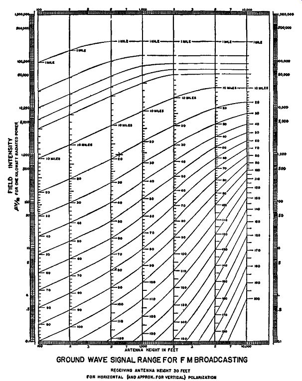
Fig. A-5. Chart by which the distance to a particular contour from the
transmitting antenna can be determined.
If we desire to find what height the antenna should be to give a field intensity of 1000 µv/m at the 20-mile contour, the following procedure is used. Place a ruler across the page so that it lines up with the 1000 markings of both the right and left hand columns. Find the 20-mile contour line and pivot the ruler until it is vertical (parallel to the other vertical lines); the point where it intersects the "antenna height" (abscissa of the graph) is the required height. In this particular instance, for 1000 µv/m and a 20-mile contour, the antenna height is found to be 600 feet.
Remember that this example is for 1-kw radiated power. To use this chart for a radiated power of 100 kw, the values of field intensity should be multiplied by 10, with all else remaining the same. To use this chart for a radiated power of 10 watts, the values of field intensity should be divided by 10. In other words, to use the chart for a radiated power other than 1 kw, multiply the values of field intensity by the square root of the ratio of the desired power to 1 kw.
I-F RESPONSE CURVES
In visual alignment the amount of deviation of the FM signal generator determines how much of the response curve will appear on the screen. It was stated in Section 8 that as wide a deviation as possible should be used in order to see the complete response curve under test.
But some FM signal generators are unable to produce sufficient deviation. Insufficient deviation will cause only part of the response curve to appear. This need not be detrimental to the alignment procedure if one understands the response curve.

Fig. A-6. IF response curves under different amounts of deviation. The
dots on each curve mark the limits of the portion of that curve appearing
in the succeeding curves.
In Fig. A-6 four i-f response curves are illustrated. These drawings represent true pictures taken under experiment, but it should be re membered that the sharpness of the curves and the selectivity requirements differ for different i-f systems. Each is taken from the same i-f network but with different amounts of peak-to-peak deviation. In part (A) the deviation was 600 khz, more than sufficient to show the complete response curve including the bottom. In part (B) the 450- khz deviation was still sufficient to obtain a complete curve. In parts (C) and (D) the deviations were 300 khz and 200 khz respectively. As the deviation decreased, the sides of the response curve became smaller.