TECHNICAL workers in electronics frequently use meters without stopping to think what the meters are and what they are supposed to do. It is quite true, of course, that as the purpose of a meter is to give an indication of circuit conditions, mere observation of the meter reading ought to suffice. For example, it may be argued that a car driver need not know how his speedometer works since all he wants to know is the speed of the car, but it doesn't concern him very much whether the speedometer shows 50 or 55 mph, for the instrument may be inaccurate, the drive gearing may be wrong for the size of tires used and the tires themselves may not be inflated to the correct pressure. In electronics measurements, one has to be more careful about the accuracy of readings. Sometimes the reading may be wrong due to an inaccurate meter and sometimes the wrong answer will be given by an accurate meter because it is improperly used. Such unhappy cases are avoided by having some knowledge of meters and other indicators and how they work.
Meters for voltage, current and resistance
Voltmeters, ammeters and ohmmeters are all ammeters because they measure current; their scales may be calibrated in volts or ohms but they are still ammeters. These remarks apply, of course, to the usual moving-coil meters on every service technician's bench. There are other meters which are not ammeters, such as electrostatic voltmeters for measuring high voltages; these are pure voltmeters.
Moving coil meter
Current passing through the pivoted coil of the meter (to which is attached the pointer) creates a magnetic field which is acted on by the magnetic field of the permanent magnet built into the meter. The meter, in fact, is an electric motor but without a commutator because continuous rotation is not required. The armature is restrained by the springs controlling the movement (these springs return the pointer to zero in the absence of an applied current) and the angular displacement of the armature is proportional to the current passing through its coil. Such a meter will give a readable deflection on de only.
To use the meter as a voltmeter a fixed resistance R is connected in series with the coil, as shown in Fig. 1101-a. Application of a voltage to the two components causes a current to pass through the circuit of a value: V l=--- R+Ra where Ra is the internal resistance of the meter. As R is increased so the current through Ra falls-hence it can be considered a multiplying resistance. If various values of R are selected by a switch, the meter circuit becomes a multirange voltmeter.
In Fig. 1101-b, absence of shunt resistor R would cause the whole current to pass through the meter, which is now acting as a straight ammeter. The internal resistance of the meter will limit the current passing through it and the resistor. If the current is greater than the meter can show, then the meter is shunted by R, which diverts a proportion of the current. Strictly speaking, R is still a multiplying resistance since it permits the meter to register a higher current than is possible in its absence, but it is usually called a shunt.
Ac meters
For measuring ac voltage and current there are several types of meters, but it is now customary to use a de moving-coil meter in conjunction with a copper oxide rectifier, as in Fig. 1101-c. The current-carrying capacity of the meter is determined by its full scale deflection. But the rectifier also has a maximum current capacity, and if the resistance of the meter is too high (or a fuse in the meter is blown so that the meter is open-circuit) the rectifier will be destroyed, owing to the full circuit voltage being applied to it. Voltage multipliers can be inserted in the rectifier circuit at R, but increased current ranges can only be provided by using an input current transformer, shown dotted, if a linear scale is to be maintained.

Fig. 1101-a, -b. To use the ammeter as a voltmeter (left) a series resistor
is inserted. The meter range is extended (right) through the use of a
shunt resistor.
If the dc scale of the meter is used, the current registered will be the mean value ac current passed. But what is wanted is the rms value, which is higher than the mean value in the ratio of 1.11; a 100 µ.a-scale deflection will represent an rms current of 111 µ.a. The scale will be linear for ac as well as de except for very small currents, when the rectified alternating (direct)current tends to be proportional to the square of the alternating current. This ...

Fig. 1101-c. Dc meter, in conjunction with rectifiers, can be used to
measure ac voltage and current.
... causes a closing up of the scale at the low end. This is why the rectifier cannot be expected to give linear rectification if it is shunted by resistance for the measurement of heavy currents, which explains the use of a current transformer for this purpose.
Similarly, linear scales for low ac voltages can be secured only by using an input stepup voltage transformer.
Given a high-grade rectifier, ac meters of this type can be de pended on for good accuracy with sinusoidal inputs up to 100,000 hz. Thereafter the response will fall off until at 1 mhz the reading will be 20% low. For audio measurements, therefore, the meter can be taken as accurate, provided the current measured is sinusoidal. In-phase second-harmonic distortion will give a reading which is low up to about 2%; in-phase third harmonic will give a meter error up to +5%, but third harmonic 180° out of phase will give a reading up to -9% low. Rectifier instruments should not be used for measurement of distorted ac waveforms.
Measuring resistance
By Ohm's Law we know that R (ohms)= E (volts)/ I (amperes). This applies also to ac provided it is remembered that the resistance may consist of noninductive, non-capacitive resistance plus the impedances of any inductances and capacitances in the circuit, the values of which depend on the frequency of the ac. So far as de is concerned, it is necessary only to measure the voltage applied across a resistor and divide by the current passing through it to get the value of the resistance of such a circuit as is shown in Fig. 1102-a, but a word of warning is necessary. If the current passing through the voltmeter is appreciable as compared with that passing through R, then the reading will not be accurate. There fore, the voltmeter must be connected on the battery side of the ammeter. If, however, the resistance of the ammeter is appreciable as compared with R, then the voltmeter must be connected as shown dotted, for it is necessary to know the voltage actually applied to R.

Fig. 1102-a, -b. Measuring resistance by voltmeter-ammeter method (left)
or by using an ohmmeter (right).
On this simple basis an ohmmeter can be constructed. The battery voltage can be fixed (and is invariably connected inside the instrument case), but as the battery will deteriorate with age, some compensation must be provided for this. In the circuit of Fig. 1102-b, if the terminals Rx are short-circuited, the only resistance in the circuit is R plus the internal resistance of the meter. Accordingly R can be adjusted to give full-scale deflection and this point will indicate zero ohms across terminals R . If the short is removed and a resistor is connected across the terminals, the current passing through the meter will fall and the higher the resistance, the smaller will be the deflection .

Fig. 1103-a. Wheat stone bridge for measurement of dc resistances.

Fig. 1103-b. Ac bridge.
A resistance scale can be drawn on the meter which will read from right to left, the reverse of current and voltage readings, and the scale will also become increasingly crowded toward the left.
The useful range can be extended by having several resistance ranges, and the multiplier this time requires a greater voltage from the battery, so that a measurable current can be passed through a higher value of resistance.
Naturally it is desirable that the scales should have a simple multiplying factor, say 10 times, so that only one resistance scale need be used. This calls for quite careful design of the complete meter. On any range the preliminary routine must be to short the resistance terminals and adjust zero (full-scale deflection) before making any resistance measurements.
Accurate measurement of current and voltage is merely a matter of selecting a suitably accurate meter, but there is no such thing as a highly accurate ohmmeter because of the bad scale characteristics. Accurate measurement of resistance is best done on a bridge.
Bridges
The circuit of Fig. 1103-a shows the Wheatstone bridge for measurement of de resistances. R1 and R2 are usually banks of precision resistors with values of 1, 10, 100 and 1,000 ohms; R3 is a decade resistance box with a minimum value of I and a maxi mum value of, usually, 11,111 ohms. Galvanometer G is used as an indicator of balance. If the ratio of the unknown resistance Rx to the variable resistance R3 is the same as the ratio of R 1 and R2 the bridge will balance. Therefore, if R1 and R2 have the same value, the value of the unknown resistance will be found by determining what value of R3 is needed for balance. If Rx is out side the limits of value of R3, balance can be found by changing the ratio of R1 to R2.
For all cases: R1 R =-X R3 x R2
The limitations of the Wheatstone type of bridge are found in measuring low resistances, because of the resistance of the leads and contacts, and in very high resistances, because of the very high R1/R2 ratio required, and the fact that no galvanometer has a sufficiently high resistance to match the bridge resistance. For such cases a de vacuum-tube voltmeter is a better indicator and, of course, the battery voltage can be raised. Low resistances are best measured on a Kelvin bridge.
An ac bridge has basically the same form, as shown in Fig. 1103-b, except that an oscillator is used as the energizing source and a null indicator (headphones, c-r tube or ac vacuum-tube voltmeter) for balance. Here, as before, the bridge is balanced when Z1/Z2 = Z3/Z4, but attention has to be paid to the nature of the impedances. If Z1 and Z2 are purely resistive, as they often are, then Z3 and Z4 must both be identical kinds of impedance: if Z3 is inductive, Z4 must be inductive; if Z3 is capacitive, Z4 must be capacitive. A complete bridge requires, therefore, standard resistors, capacitors and inductors to be used for Z4 where resistance, capacitance and inductance have to be measured. The other extra feature is the potentiometer across the oscillator labeled "Wagner ground." Both oscillator terminations have capacitance to ground which may make balance impossible; the Wagner ground enables a balance to be secured without interfering with the operation of the bridge.
There are many types of ac bridge, each having been devised for some special application. Standard inductors, for example, are costly and cumbersome and can be avoided by using a Maxwell bridge. This compares unknown inductors with standard capacitors using resistors for Z1 and Z4, with capacitance and resistance in Z2. The Wien bridge measures capacitance in terms of resistance and frequency or frequency in terms of the other quantities.
Details of these and other specialized types can be found in any standard textbook on ac bridge methods.
Vacuum-tube voltmeters
To measure the actual de voltage on the plate of an amplifying tube, we must remember that the plate current passes through the plate-load resistor and also the decoupling resistor, if one is in the circuit. If an ordinary moving-coil voltmeter is used to measure this voltage, the current drawn by the voltmeter will cause a potential drop across the load and other resistors and give a grossly inaccurate reading. The error will be diminished if the meter only draws a small current. Meters of the type described as "20,000 ohms-per-volt" give a reasonably correct measurement of plate voltages for general service work. Some modern meters have sensitivities up to 100,000 ohms-per-volt. But for design purposes the accuracy is not good enough-the meter should draw practically no current from the circuit under investigation. A vacuum tube voltmeter is such a device.
Vacuum-tube voltmeters are of differing types, some for dc measurements, some for ac; combined instruments contain facilities also for measuring resistance. As the application of the vtvm to the circuit has virtually no effect on its behavior, it is a very simple matter to check all tube voltages and also gain, stage by stage. An audio oscillator provides the input signal for the amplifier, adjusted to the rms value postulated by the design. Voltage amplification is then measured throughout the amplifier by probing at successive grids and plates. If the oscillator input is held constant and varied throughout the frequency range of the amplifier, it is possible to take a response curve of the amplifier stage by stage, thus locating at what point, if any, the performance is defective. Response measurements of amplifiers should, as pointed out in an earlier section, be taken with a resistive output load.
Oscillators, oscilloscopes and other devices
No audio design or measurement work can be done without a signal source. An audio oscillator with a frequency range of about 30 to 30,000 cycles is an essential piece of equipment for the audio engineer. Various types are available and the comparatively recent R-C oscillators are considerably simpler and cheaper than the much older beat-frequency kind. The requirements are that the output should be quite sinusoidal at all frequencies; that the stability of frequency should be reasonably good; that the output should be capable of suitable attenuation. A useful feature is the ability to switch from sine-wave output to square-wave when de sired. The square-wave output is generally achieved by using a clipped sine wave; for amplifier testing this can be considered quite good enough for all ordinary purposes.
Waveform investigation is impossible without a cathode-ray oscilloscope, and the larger the tube the greater the ease of examining the waveform. ·when the output of the amplifier is being examined, it is desirable to make a continual check that the input is true to specifications. This can be done by having an oscilloscope on both input and output. Separated oscilloscope traces are not easy to compare, so the use of a double-beam oscilloscope has great advantages in direct comparison. The input waveform can be given the same amplitude on the tube as the output by suitable adjustment of the internal amplifiers of the oscilloscope. Double beam oscilloscopes are not so common as to be easily come by, but an ordinary oscilloscope can be converted into a pseudo double beam instrument by using an electronic switch which switches the oscilloscope from the input to the output so rapidly that the tube screen persistence gives a continuous picture. A separate provision for adjusting the compared voltages is provided for in the electronic switching circuit.
Amplifier frequency response
The frequency response of an amplifier can be displayed on the c-r tube by using a sweep generator to sweep the whole frequency range sufficiently rapidly to give a steady trace on the screen. In this way adjustments to improve the frequency response are instantaneously observable. But this will not at the same time check for waveform distortion; an amplifier must be checked separately for frequency response and freedom from distortion.

Fig. 1104. Block diagram of layout for measuring performance of an amplifier.
Harmonic analyzers are desirable but not essential pieces of equipment in an audio laboratory for the amplifier designer's task is not to produce certain percentages of harmonic distortion but to eliminate it as far as possible. Knowledge of what various wave forms mean as to harmonic content is necessary to interpret the pattern and a selection is given.
Measurement techniques
Testing an amplifier for overall performance should be done on the basis of the amplifier delivering its maximum undistorted output. Performance under any other conditions is quite misleading.
In the block diagram of Fig. 1104 an audio oscillator is shown energizing the amplifier under test. If the oscillator has no output meter, an ac (rectifier type) voltmeter to measure the input volts must be added as shown. Every component and lead attached to the input of the amplifier must be properly shielded, otherwise hum will be introduced which will nullify the measurements.
A resistive load is connected across the output and this resistance must be capable of dissipating the full power output of the amplifier. This would suggest a wirewound resistor, but as this is inductive its impedance will vary with frequency. The load resistor is best made up of paralleled composition resistors of the highest ratings obtainable, unless, of course, noninductive wire-wound units are available (easily made by winding on to a former a doubled resistance wire so that the two free ends are at the same end of the former).
First test for stage gain, at, say, 1,000 cycles. Set the oscillator to this frequency and the oscillator output to give the designed rms input to the amplifier. Using a vtvm, touch successive grids and plates up to and including the output-stage grid circuit to make sure that the amplification per stage is as designed. The value of the load resistor is known and if the voltage across it is taken on an ac voltmeter (again a rectifier type) the current can be calculated by I = E/R, and the output watts roughly by W = I X E. If the watts produced are too high, then there is too much gain in the amplifier; if too low, the gain is not enough. Generally speaking a ...

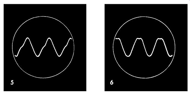
---------- Trace 1) Sine wave; Trace 2) 15% 2nd harmonic +90° out
of phase.
.... little too much gain is usually of no importance; too little gain can be very tiresome. (These remarks must be modified by the feed back setting.) An oscilloscope should now be connected as shown in Fig. 1104.

------- Trace 3) 15% 2nd harmonic -90° out of phase; Trace 4) 30%
2nd harmonic in phase.
For a single-beam type, a switch should be included to permit examination of the input and output waveforms; a double-beam oscilloscope will show input and output simultaneously. Check that the output at full watts is sinusoidal. At the same time note the voltmeter reading and put index marks on the scope reticule to denote the vertical height of the wave pattern. The output volt meter can now be removed. Without bothering to reset the time base of_ the oscilloscope for other frequencies, sweep the oscillator down to the lowest frequency and up to the highest the amplifier is designed to reproduce. Non-setting of the time base gives a muddled oscillogram but makes it easier to see if the height has varied at all. As the height of the pattern is proportional to the voltage it is a very simple matter to plot output voltage against frequency and so make a quick response curve of the amplifier. If the frequency response is what the designer intended, examination of the waveform at all frequencies can now be undertaken.
Keeping the input constant at the prescribed voltage and using the oscilloscope time base in the normal manner, check that a sine wave output exists at all frequencies. If everything appears to be in order, the audio oscillator can now be switched to square wave output and the examination repeated. It is necessary to point out that a perfect square wave cannot be expected all over the frequency scale. At the low end, departure from the square is to be expected, but certain features of waves that are not square cannot be passed (see the waveforms given in this section). At high frequencies the thing is impossible unless the amplifier has an infinitely wide response. If the designed response of the amplifier is to be flat up to 50,000 cycles, the square wave will begin to lose its squareness at about 5,000. A square wave consists of a fundamental and an infinite series of harmonics; absolute squareness is not required, fortunately, but enough harmonics must be amplified to give reasonable squareness. If the amplifier cuts off at 50,000 cycles and the square-wave input has a frequency of say, 30,000, it will be obvious that not even the second harmonic will be amplified. In practice the oscilloscope will show very nearly a sine wave at all square-wave inputs above about 15-20,000 cycles.
But note particularly that as the square wave degenerates gradually into a sine wave, it must not, at some point, take on an irregular form for this will show that the amplifier is distorting transients very badly. The transition must be smooth and gradual.
Where the secondary of the output transformer of an amplifier provides alternative taps for speakers of various impedances, the tests given here must be repeated for each tap, using the appropriate load resistance.
Interpretation of waveforms
The oscilloscope will display any distortion present in the out put of an amplifier, but if the screen is small and the trace not finely focused, distortion which would be audible to a trained ear may not be perceptible to the eye. Some skill is needed to interpret what is seen on the screen. The waveforms of typical traces should be studied in conjunction with these notes.
Small amounts of harmonic distortion will not be seen except on a 5 or 7 inch tube with very good focusing, and even then it may be desirable to have a pure sine wave inscribed on the re movable tube reticule for comparison purposes. If such is used, then the horizontal and vertical shifts and amplifiers must be adjusted so that a sine-wave input coincides with the reference waveform. This refinement can, however, be dispensed with (and would be out of place with a small oscilloscope) if the amplifier under test is driven to overload. The increased harmonic distortion will then be readily seen and its nature determined. Such traces would not be correct for the amplifier under normal operating conditions, but they will indicate wherein the suspected impure sine wave departs from the perfect form.
Trace 1 shows a sine wave; with a small oscilloscope it may be desirable to alter the sweep frequency so that only one complete wave is displayed at any frequency; this will make it easier to spot departures from the perfect form, but involves considerable adjustment to the time base. As a general rule not more than three complete waves should be displayed otherwise it will be impossible to detect irregularities in the waveform except at maximum and minimum points; the accompanying traces generally give two waveforms. The appearance of a pure sine wave should be memorized for the particular oscilloscope in use, for faults in the oscilloscope may distort the trace. The instrument should, of course, be free from innate distortion, but if it is not quite perfect, a note should be taken of the shape of the sine wave trace.
------------- Trace 5) 30% 211d harmonic 180° out of phase; Trace
6) 30% 2nd harmonic +90° out of phase.
Second harmonic distortion
5% second harmonic distortion will hardly be perceptible at any phase displacement of the harmonic. If the second harmonic is out of phase with the fundamental there will be a gradual widening of the top or bottom of the waveform as shown in traces 2 and 3 which represent 15% second harmonic with phase differences of +90°. Even harmonic distortion is present in single out put tube amplifiers and in out-of-balance push-pull amplifiers to a small extent. Traces 2 and 3 show the result of overloading (as, in fact, do all the other traces) that produces the characteristics of second harmonic distortion.

------------- Trace 7) 30% 2nd harmonic -9.0° out of phase; Trace
8) 15% 3rd harmonic in phase.

---------------- Trace 9) 15% 3rd harmonic +90° out of phase; Trace
10) 15% 3rd harmonic -90° out of phase.
If the second harmonic is in phase with the fundamental or 180° out of phase (being the reciprocal of in phase, as -90° is the reciprocal of +90°) the sides of the wave will begin first to lean to one side and straighten and then take on a curvature opposite to that of a sine wave. If the harmonic is in phase, the lagging side will begin to kink, if 180° out of phase the leading side will kink. Trace 4 shows 30% second harmonic in phase with the fundamental; trace 5 shows 30% second harmonic 180° out of phase. If the second harmonic is 90° out of phase, but with 30% amplitude, the tops and bottoms· will flatten as shown in traces 6 and 7, these being emphasized conditions of traces 2 and 3.
Third harmonic distortion 5% third harmonic in phase with the fundamental will need careful observation to see the difference from a sine wave, the tops and bottoms are both slightly rounded, but if 180° out of phase, the sides of the waves will be straighter. Notice that in-phase third harmonic tends to broaden both tops and bottoms, in contrast to second harmonic which broadens tops or bottoms. As the amplitude is increased to 15%, the in-phase third harmonic gives the shape at trace 8; an increase to 30% produces trace 11. This follows a similar sequence of flattening tops or bottoms of the second harmonic ±90° out of phase, but the flattening starts earlier.
Third harmonic 180° out of phase gives straighter sides, as has been stated, and these develop into the characteristic shape of trace 12, which represents 30% third harmonic. Note particularly, however, that the straight sides perceptible with 5% third harmonic are quite symmetrical when the harmonic is 180° out of phase, for even with the kinks of trace 12 each half cycle is sym metrical. However, if the third harmonic is ±90° out of phase the straight sides will not be distinguishable from excessive second harmonic in phase for small percentages.

------------Trace 11) 30% 3rd harmonic in phase; Trace 12) 30% 3rd harmonic
-90° out of phase.

------------ Trace 13) 15% 4th harmonic in phase; Trace 14) 15% 4th
harmonic +90° out of phase.
An increase of amplitude reveals the essential differences in traces 9 and 10, which display 15% third harmonic 90° out of phase. In the second harmonic, traces 4 and 5, the kink is in the middle of the side of the wave; with third harmonic it is nearer the top and bottom. Also traces 4 and 5 represent 30% second harmonic while 9 and 10 represent 15% third harmonic; distortion becomes evident much sooner with third harmonic to the ear as well as to the eye.
Fourth harmonic distortion
5% of fourth harmonic is distinctly noticeable. Traces 13 and 14 show 15% in phase and +90° out of phase; the traces would be reversed for reciprocal harmonic content. Fourth harmonic would be present in single tube output stages, but generally in much smaller percentage. A combination of 5% second and fourth harmonic would give a trace somewhat similar to those of traces 13 and 14. These traces obviously would not appear when investigating a properly balanced push-pull amplifier.
Fifth harmonic distortion
Fifth harmonic is soon perceived. Trace 15 gives the trace for only 5% fifth harmonic in phase with the fundamental; with in crease, the form in trace 16 develops, which shows 15% of fifth harmonic. If the fifth harmonic is 180° out of phase with the fundamental, the patterns of traces 17 and 18 appear, representing 5% and 15% respectively. Note that the form of trace 14 is repeated in trace 18 except that the flattish bottoms of trace 14…

----------- Trace 15) 5% 5th harmonic in phase; Trace 16) 15% 5th
harmonic in phase.
… appear also in the tops of trace 18 as well as the bottoms; as a similar relation exists in traces 6 and 8 it will be seen that there is a "family likeness" in odd harmonics as there is in even harmonics.

-------------- Trace 17) 5% 5th harmonic 180° out of phase; Trace
18) 15% 5th harmonic 180° out of phase.
Combinations of even harmonics (as also combinations of odd harmonics) display the family pattern but with less total harmonic content than the traces from separate harmonics, conforming to the generally recognized principle that wide range reproduction must avoid high harmonic distortion; a wide range speaker very quickly reveals distortion in an amplifier of limited performance.
Second plus third harmonic distortion
This combination is always present with single tetrode output stages. 5% of second and third is shown in trace 19 (both in phase with the fundamental) and if the amplitude of the third harmonic is greater than that of the second, as is usual with tetrodes, the very characteristic shape of trace 20 develops. Increasing the

-------------- Trace 19) 5% 2nd harmonic in phase and 5% 3rd harmonic
in phase; Trace 20) 5% 2nd harmonic in phase and 15% 3rd harmonic in
phase.

--------------- Trace 21) 5% 2nd harmonic in phase and 30% 3rd harmonic
in phase; Trace 22) 5% 2nd harmonic in phase and 30% 3rd harmonic 180°
out of phase; Trace 23) 15% 2nd harmonic -90° out of phase and 15% 3rd
harmonic in phase; Trace 24) 5% 3rd harmonic in phase and 5% 5th harmonic
in phase; Trace 25) 5% 3rd harmonic in phase and 5% 5th harmonic 180°
out of phase.

------------------ Trace 26) 5% 3rd harmonic 180° out of phase and
5% 5th harmonic in phase; Trace 27) 5% 3rd harmonic 180° out of phase
and 5% 5th harmonic 180° out of phase; Trace 28) waveform when amplifier
is set to maximum undistorted output; Trace 29) slight overloading; Trace
30) more overloading.
... third harmonic content still more produces trace 21, which differs from trace 11 in that the two peaks are not the same height.
If the third harmonic only is out of phase with the fundamental, trace 22 is produced, but this is not the same as trace 12, for the halfway kinks are not symmetrical as they are in trace 12. If the second harmonic is 180° out of phase and the third harmonic is in phase, traces 19 to 22 are reversed. Trace 23 represents 15% each of second and third harmonic, and differs from trace 6 in that the bottom troughs are wider.

-------------- Trace 31)
Severe overloading; Trace 32) square wave.
----------------- Trace 33)
Effect of long time constant on a square wave; Trace 34) Effect of short time constant on a square wave.

--------------------- Trace 35)
Effect of an amplifier (with good response) on a square wave; Trace 36) Effect of an amplifier (with bass attenuation) on a square wave.
Third plus fifth harmonic distortion
This combination is present in all push-pull tetrode amplifiers when overloaded. This type of distortion is soon seen and heard.
Trace 24 shows 5% of each in phase with the fundamental; trace 25 when the fifth harmonic is 180° out of phase; trace 26 when the third harmonic is 180° out of phase; trace 27 when both the third and fifth harmonics are 180° out of phase. If either harmonic is only 90° out of phase, the tops and bottoms will be tilted to the right or left. It will be noticed that the divergence from the sine wave form is less when both harmonics are in phase with each other even if out of phase with the fundamental. As phase shift is directly associated with attenuation, in-phase conditions are se cured by having an amplifier with wide frequency response.
General observations
If an amplifier under test is set to maximum undistorted output power and the output applied to the oscilloscope, the trace will appear as in 28. The oscilloscope vertical amplifier must at no time be overloaded itself and is best set to give a trace not more than about one third of the screen diameter in height. If, now, the input to the amplifier under test is increased, distortion will begin to appear, as in trace 29; with further increase of input the trace will change to 30 and then 31, which is a fairly good imitation of a square wave; this denotes very considerable distortion. An almost perfect square wave can be obtained from a fundamental and twelve odd harmonics, and traces 30 and 31 might be considered roughly as a sort of summation of all the earlier traces. This square-wave output can be used as a means of checking the performance of the amplifier under normal conditions by injecting a square wave from a suitable input oscillator.
Square wave testing

-------------- Trace 37) Effect of an amplifier (with treble attenuation)
on a square wave, typical of an amplifier without negative feedback,
at 3,000 hz.

----------------- Trace 38) Effect of an amplifier without negative
feedback on square wave at 10,000 hz; Trace 39) Effect of an amplifier
with negative feedback on square wave at 10,000 hz.

------------------ Trace 40) Parasitic oscillation revealed by square
wave; Trace 41) Two voltages in phase; Trace 42)
Two voltages Jo• or JJO• out of phase; Trace 43)
Two voltages 60° or J00° out of phase; Trace 44) Two voltages 90° or 270° out of phase.
The oscillator should be applied to the oscilloscope for checking; trace 32 gives the appearance of the square wave on the screen.
An amplifier without feedback can hardly be expected to give a true square wave at any frequency, for if a simple R-C coupling is inserted between the oscillator and the oscilloscope, a trace like 33 will be obtained with a long time constant and one like 34 for a short time constant. It might be supposed, therefore, that a complete amplifier with perhaps three R-C couplings will look very bad indeed. In practice it is not quite like this, for the trace depends on the phase shift at various frequencies and phase shifts will sometimes cancel.
First take an amplifier without feedback. At 50 hz the trace will appear as in 33 if the bass response is exceptionally good; if poor, like 34. In general it will appear like trace 36. At the usual mid-frequency, 1,000 hz, where the amplifier is usually flat for some octaves below and above, there will be the nearest approach to a square wave, but with some rounding of the leading upper and lower corners. At about 4,000 hz, the shape will have changed to trace 37, owing to a loss of high harmonics, and at 10,000 hz the output will be nearly sinusoidal, as in trace 38.
Addition of the right amount of feedback will secure a trace like 35 at 50 hz. As the frequency rises the form will change to a perfect square wave at 1,000 hz which should be maintained until at least 3,000 hz. Thereafter the shape will gradually spread until at 10,000 hz the trace of 39 will be developed. After that, the squareness will depart until a sine wave is reached.

-------------- Trace 45) Two voltages 120° or 240° out of phase.
The oscilloscope is unquestionably the surest way of setting the amount of feedback. If the feedback is too great, motorboating will start, indicated by the pattern jumping up and down on the screen. Reducing the feedback will increase the gain and increase harmonic distortion. Adjustment of the feedback is probably most easily settled by driving the amplifier into overload and increasing the feedback until gain and distortion is reduced to the desired level. Such adjustments are best carried out using a sine-wave in-put; but when the best setting is thought to have been reached it is necessary to switch to square-wave input, for the amplifier may be only "conditionally stable" and may break into oscillation by the shock excitation of the transient front of the square wave. The amplifier should also be switched off and the tubes allowed to cool,

--------------- Trace 46) Two voltages 150° or 210° out of phase.
... then switched on again to see if there is instability on warming up.
If there is, the margin of safety is inadequate.

------------------ Trace 47) Two voltages 180° out of phase.
Distortion of the waveform as in trace 40 is known as ringing. It is due to parasitic oscillation and must be located and cured.
Phase measurement
The oscilloscope is the most convenient instrument for displaying the phase relationships of two voltages. One voltage is applied across the horizontal plates, the other across the vertical plates.
The time base is not used. The horizontal and vertical amplifiers should be adjusted so that the spot displacement on the tube is equal on both axes. When the two voltages are in phase, the trace is as shown in 4 I; when 180° out of phase, trace 4 7 applies. The circular trace 44 indicates that the two voltages are 90° or 270° out of phase; an elliptical trace indicates intermediate phase differences. Trace 42 represents 30° or 330°; 43 is for 60° or 300°; 45 shows 120° or 240° and 46 is 150° or 210°. The phase/frequency characteristic of an amplifier can be easily taken by connecting the input of the amplifier (output of the sinusoidal oscillator) to the horizontal plates of the oscilloscope, and the output to the vertical plates. The oscillator is then run over the frequency scale and the phase shifts of the whole amplifier noted for each frequency. This provides the preliminary information before planning feedback circuits to improve the response.
Perfection of phase inversion stages can be checked by connecting the output-tube grids to a horizontal and vertical plate, the other plate terminals being common grounded to the amplifier ground. The trace should be exactly as 4 7; if not, the parameters of the phase inversion stage must be modified until the phase in version is exactly 180°.