A close look at the up-to-date measurement techniques that underpin HIGH FIDELITY'S speaker testing program.
by Emil Torick
[Emil Torick supervises the HIGH FIDELITY test program at the CBS Technology Center, where he is director of audio systems technology. He is president-elect of the Audio Engineering Society and maintains an avocational interest in music as a symphony violinist and organist/choir director.]
"IT TALKS. IT WHISPERS. IT SINGS." Thus pro claimed an advertisement, nearly a century ago, for one of the earliest commercial models of the Edison phonograph. It would have been difficult to make separate technical performance tests on the rudimentary horn loudspeaker of that device, integrally connected as it was to the rest of its mechanical reproducing apparatus. But it is undoubtedly true that it did talk, whisper, and sing-as well as shriek, grunt, scratch, and create myriad other sounds. Today, when we examine high fidelity loudspeakers, we hope that they will do none of these things, that they will not inject their own personalities into the reproduced musical performance, that they will simply and accurately convert an electrical signal into its exact acoustical equivalent. That is our hope, and to a first approximation all modern loudspeakers achieve that goal. Against more exacting criteria, however, significant differences immediately become apparent. This, then, is the purpose of the HIGH FIDELITY speaker test program-to identify and quantify those essential performance characteristics that distinguish notable reproducing systems from ordinary ones.
The accomplishment of this task requires the co operative efforts of skilled engineers and critical listeners. At the laboratories of the CBS Technology Center in Stamford, Connecticut, each speaker system is subjected to a battery of technical measurements intended to "exercise" it both under normal operating conditions and near the limits of its capabilities. After the measurements have been completed, and the resulting data sorted and analyzed, the "golden ears" of the HF editors go to work in the listening room in Great Barrington, Massachusetts. No significant performance detail is overlooked.
Indeed, the human ear is in some respects still the most sensitive piece of test equipment yet invented. It is possible to hear certain defects that are beyond the resolution capabilities of today's electronic test instrumentation. Conversely, the electronic tests provide a significant degree of repeatability and quantification of performance results. Furthermore, as currently implemented at CBS, the technical measurements are intended to predict what a listener will hear. Thus the sub sequent listening tests provide a corroboration as well as an interpretation of the lab data.
Not all loudspeakers are designed to provide truly "high fidelity" response. Musical instrument speakers are a good example. The designer of an electric guitar system or an electronic organ considers the loudspeaker to be an integral part of the tone -generation system of his product. Nonlinear response that would produce distortion in a phonograph may be a source of the coveted "distinctive" sound in a musical instrument. In these applications, the paramount factors may be power -handling capability and frequency range, rather than such attributes as frequency response and pulse response. For high fidelity applications, however, all are important, and a worthwhile test program must provide a complete characterization of loudspeaker performance.
Frequency Response
The first requirement of any audio reproducing apparatus is that it respond to all frequencies of excitation in a similar manner, unless such response is intentionally altered (as in an equalizer).
Amplifiers have the easiest time of this, transducers a more difficult one. In a phonograph cartridge, for example, the various moving elements of the mechanical system exhibit their own resonances, which may interact with record groove modulations to produce a less -than -perfect response. In a loudspeaker system the goal becomes even more difficult to achieve. There are the same constraints associated with moving parts, but to this we must add the effects of the cabinet, the interactions of the low, midrange, and high frequency drivers (at various points in space), and the environmental effects of the listening room itself.

Fig. 1: On-axis pure tone response

Fig. 2: Mike array in anechoic chamber.
This latter effect creates a salient problem in testing a loudspeaker. For a test procedure to be universally useful, the reported results must not be dependent on the response in any single environment. The data must be repeatable; they must provide a basis for comparison between various system approaches (for example, between direct radiation and reflection); and they should in general attempt to characterize all systems fairly. The listening room, then, is an uncontrollable factor facing both the designer and the evaluator of a speaker system. The designer may specify that a speaker should be mounted a certain distance from a wall to provide correct back reflections. He may specify that corner placement is essential to achieving adequate low -frequency response, or he may recommend a minimum height off the floor to prevent "boominess." What he does not specify is the room itself, obviously because one must accept what is available in this regard and also because room response cannot be accurately analyzed. As Frederick V. Hunt, head of the Acoustic Research Laboratory at Harvard University, said just a few months before his death in 1972, "We have finally learned to solve the equation of an empty, plain, hard -walled, rectangular room. But let someone put a single chair in that room, and we do not yet have the means to predict its effect." Because of all the variables attendant in making loudspeaker measurements in a conventional room, so-called free-field measurements are taken instead. In free-field measurements, the boundaries of the room are removed--acoustically speaking. These tests can be performed outdoors high above any reflecting surfaces but are more conveniently performed in an anechoic chamber.
Literally a room without echo, the anechoic chamber has walls that are highly absorptive acoustically. Since there are no reflections, there are consequently no reinforcing (in -phase) nor canceling (out-of-phase) interferences.
At the CBS Technology Center, the anechoic chamber is approximately 16 by 9 by 15 feet high and is constructed of 8-inch block walls with an 8 -inch concrete floor and a 3-inch precast ceiling.
The entire assembly is suspended top and bottom by springs at approximately a 3-Hz resonance to isolate the room effectively from external noise sources. Acoustic absorption is obtained with 45 -inch glass-fiber wedges that line the entire interior surface. An open metal-grille platform supports personnel and equipment without affecting the absorption of the wedges or causing significant reflections.
The basic response measurement made on all loudspeaker systems is a pure -tone frequency sweep at a power level low enough to minimize distortion. A microphone, with calibration trace able to the U.S. National Bureau of Standards, is mounted 1 meter away from the front geometrical center of the speaker cabinet. The measurement registers automatically on --a chart recorder synchronized to a variable-frequency oscillator. Fig. 1 shows a typical charted response. While this particular graph does not tell much about the absolute performance of the speaker itself, it does give a good picture of the relative response of any equalization controls (which are provided for the highs only on this example).
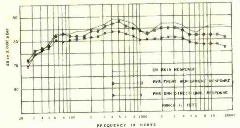
Fig. 3: Third-octave -band noise response

Fig. 4. Measured impedance curve
More meaningful frequency-response measurements are made using noise as the energizing signal. Random noise that has equal energy at all frequencies is called white noise. Since it is more convenient to use one-third -octave bands of noise, we use "pink noise"--which by definition has constant energy in all bands--to effectively average out insignificantly narrow peaks and dips in the response. Three response curves are plotted: The first is analogous to the on -axis response in Fig. 1; the second represents the total power radiated directly into the hemispherical space in front of the speaker; and the third represents the total power output for radiation in all directions.
In such measurement of total power output, we employ unique electroacoustic equipment and computer aids. The Loudspeaker Power Monitor, recently developed by the CBS Technology Center, uses a special algorithm to process simultaneously the outputs of twelve individual micro phones. Fig. 2 shows these microphones in a dodecahedron array surrounding a loudspeaker in the CBS anechoic chamber. With the new test procedure, the speaker is energized with a one third-octave -band pink-noise sweep. The Power Monitor processes the microphone signals to yield the on-axis, front-hemisphere, and omnidirectional responses. The same measurement is then taken two more times, with the orientation of the loudspeaker adjusted each time so that the horizontal and vertical angles between adjacent microphones are cut into three equal parts. Thus, response data from a total of thirty-six locations about the loudspeaker are available for final computer processing and analysis. Measured frequency bands range from 20 Hz to 20 kHz-an interval encompassing thirty separate one -third-octave bands. With thirty-six locations for the omnidirectional response and eighteen locations for the hemispherical response, plus the single-location on -axis response, all times thirty frequency bands, a total of 1,650 data points must be processed. The computer handles this task easily, producing a final set of curves like the ones shown in Fig. 3.
Although the curves of Fig. 3 appear relatively easy to read, special care must be taken in interpreting them. The curve for omnidirectional response is the most significant, for it shows the total radiated energy that will ultimately react with the room to produce the final audible response. A good speaker will always show an even curve with only small peaks and valleys. Bass response should roll off smoothly, although we must recognize that radiation efficiencies at the lower frequencies will improve bass response by about 4 to 6 dB when a speaker is located in a corner of the room. Finally, a good sense of high-frequency dispersion may be gained by comparing the on-axis response with that of the other two curves. If the high-frequency contour of the on -axis response parallels that for the other two modes, the spectral balance within the treble region will remain essentially the same irrespective of listening position; if these contours converge or diverge markedly, it is an indication of irregular high-frequency dispersion--what is commonly described as "beaming."

Fig. 5: Distortion measurement system

Fig. 6: An engineer measuring distortion
Sensitivity and Impedance
You may have noticed that Fig. 3 also includes in formation about the sensitivity of the loudspeaker, which is, of course, related to its efficiency in converting electrical to acoustical energy. The vertical axis at the left margin of the chart is calibrated in units of sound pressure level (dB) to indicate what output level is produced when the speaker is driven with a voltage equivalent to a nominal 0 dBW (1 watt). Since most musical energy falls within the range from 250 Hz to 6 kHz and sound beyond these frequencies has relatively little in fluence on our basic perception of the over-all loudness of the sound, the sensitivity figure is the average sound pressure level achieved within this frequency range for a 0-dBW pink -noise input.
The figure can be used as a guide in determining how much amplifier power will be needed to drive the speaker under test to any desired sound pressure level.
Until recently the sensitivity figure was derived from the on-axis measurements. But since the important criterion is the total acoustic energy delivered into the listening room--not just that delivered in the on-axis direction-we now use the omnidirectional response data as the basis. For this reason, sensitivity ratings of front -firing speaker systems will be several dB lower than with the on-axis measurement, while designs that radiate much of their energy in other than the on-axis direction will, for that reason, exhibit higher sensitivity figures than formerly.
Wattage readings usually are not made directly; they must be inferred from a knowledge of the voltage applied and the impedance of the loud speaker. Since the actual impedance of a speaker system is not constant at all frequencies, we choose to use a factor called nominal impedance.
The determination of nominal impedance is actually the first measurement performed in a loud speaker test, for it provides the basis for level set ting in all subsequent measurements. The nominal impedance may or may not be the same as the manufacturer's rated impedance. The former value is determined quite accurately, while the latter is usually rounded out to some familiar number like 4, 8, or 16 ohms.
To determine the impedance of a loudspeaker system, we insert a high value of resistance (actually 2,500 ohms) in series between the power amplifier and the speaker terminals. Using Ohm's law, we can plot the impedance (Z) curve as a function of frequency from the voltage across the speaker and the current through the resistor. Fig. 4 shows the impedance curve for a typical multi-element loudspeaker. The rise at low frequencies is caused by the primary resonance of the woofer unit in its enclosure. (Sometimes we may see two peaks here if the system employs a vented -box configuration.) Just above the woofer resonance, the impedance curve dips to a low level. The value at this point is defined as the nominal impedance.
At higher frequencies, the impedance curve may exhibit additional peaks and valleys. Small variations are of little concern; modern amplifiers take them in stride. But significant dips below rated or nominal impedance, especially over a broad frequency range, should be viewed with some concern. The lower the actual impedance, the more risk it poses of drawing excessive current from the output of the amplifier. The situation will be aggravated, of course, if two similar speakers are connected in parallel across the amplifier.
Distortion
The measurement of distortion in any transmission or reproducing system continues to be one of the most important performance tests. In the most common procedure, distortion is measured by driving the system under test with a single tone at some specified level. The output signal is then processed, either by filtering or cancellation, to remove all traces of the original tone, and what re mains are various harmonics of the original signal, created by the undesirable nonlinear processes in the system. This remnant signal, termed total harmonic distortion, is usually expressed as a percentage of the original driving signal. In another common technique, two driving frequencies are used, either closely spaced in frequency or far apart. These signals are then processed in a manner similar to the first method to produce a measurement of intermodulation distortion-sum and difference tones of the two original signals. In the HIGH FIDELITY test program we use a third technique that is a variation of the harmonic distortion method. Most revealing for phonograph pickup and loudspeaker tests, this last method uses a sharply tuned bandpass filter to detect the level of specific harmonics-usually the second and third.
The question of which driving frequencies to use is especially difficult in a speaker test because of the uneven frequency response of most systems (remember Fig. 1!). Consider a test with a 1,000 -Hz fundamental driving frequency (whose second and third harmonics are at 2,000 and 3,000 Hz). In testing an amplifier with a ruler -flat frequency response there would be no question about the validity of the level of the 2,000- and 3,000-Hz signal components. With a loudspeaker it is an entirely different matter. These harmonics (or even the fundamental) may fall on peaks or valleys in the response or coincide with cabinet resonances or even fall where a driver is being rolled off by a crossover network. So the test results obtained clearly may be influenced by the frequency selected for the test.
In the past we have usually chosen 80 and 300 Hz as relatively useful for loudspeakers. Now, in a major step forward, and using a specially designed setup illustrated in Figs. 5 and 6, we are able to make a continuous frequency sweep for each distortion measurement. Typical results are shown in Figs. 7 and 8 for second and third harmonic measurements, respectively. The frequency scale represents the fundamental driving frequency, and the distortion level is read directly in percent on the vertical axis. Two driving levels are used-one watt at nominal impedance, and a higher level that will result in an average output of 100 dB SPL in the region of 300 Hz.

Fig. 7. Second harmonic distortion

Fig. 8: Third harmonic distortion

Fig. 9: Pulse waveform on oscilloscope
Note the widely varying distortion levels. This degree of detail would be impossible to achieve in spot frequency measurements. Note, too, the general but not consistent increase in distortion at the higher signal level. It is not unusual for distortion to be greater at lower levels. A sharp, high peak at a single frequency probably indicates a resonant buzzing of some component in the cabinet.
Power Handling
There are times in the life of any music-reproducing system when it is called upon to perform to its full limits. At such times, the stresses on each component may be quite severe, and it is especially useful to know in advance what the limitations are. Consequently, we subject a phonograph pickup to the tortuous tracking requirements of a test record and drive an amplifier hard to just be low (we hope) the point where the smoke begins to seep out. And loudspeakers get similar treatment in a combination of steady-state and pulse-power measurements.
In the steady-state measurement we determine the ability of a speaker to handle 100 watts of continuous power at 300 Hz. As the power is increased from a lower level, if the speaker begins buzzing or if the output distortion reaches 10%, we halt the test and note the power and output levels. Some times, on speakers with built-in protection, the test is halted automatically when a circuit breaker is thrown or a fuse blows. On other occasions a manufacturer may specify greater than 100 -watt capability, and that too will be checked out. In all cases, the speaker-or, rather, its output-is watched very closely to avoid the kind of overheating that would permanently damage it.
There is less danger from overheating when pulse measurements are employed, permitting even higher power levels than with the steady state measurement. It is possible to use various pulse waveforms for such a test, but the signal that best simulates the wave shapes produced by musical instruments is one that provides the simultaneous application of all frequencies in a one-third-octave band of frequencies. The actual waveform is shown in Fig. 9. It is generated by passing a square unit pulse through a one-third-octave filter, and it can be proven mathematically that all frequencies within the octave band are present and at the same power level. As the pulse signal is applied at ever-increasing levels, the output of the loudspeaker is observed on an oscilloscope. The point at which visible distortion begins to occur is considered the upper limit of the system, both in terms of peak power -handling capability and peak sound -level output.
A Final Assessment
What do the results of all these measurements mean? Only the experienced eye and ear can tell.
If it is the sound that counts and we accept the physiologist's definition of sound as "that which is heard," then the correct interpretation of the technical data requires that listening tests be performed as well. That otherwise-impressive one third -octave noise response curve may show a small level change somewhere across the frequency band. If the bass frequencies are higher in level, does this indicate a too -heavy bottom or a deficiency in highs? Only the ear can tell. Or if the highs are more pronounced in level, does this imply too much brightness or a deficiency in bass? Only the ear can tell. Is the sound quality acceptable or is that distortion peak giving an objection able edge to the sound? Only the ear can tell.
And so it goes--the happy marriage of two techniques, each complementing the other. The net result? A test report that is as accurate as state-of the-art technology permits, and one that is as meaningful and relevant as informed audition can make it.
-------------
(High Fidelity, Oct. 1977)
Also see:
Computer Technology Transforms Speaker Design (High Fidelity, Oct. 1977)