BACKGROUND
The nineteenth century was a time of great technical interest and experiment in both Europe and the USA. The newly evolved disciplines of scientific analysis were being applied to the discoveries which surrounded the experimenters and which, in turn, led to further discoveries.
One such happening occurred in 1864, when James Clerk Maxwell, an Edinburgh mathematician, sought to express Michael Faraday's earlier law of magnetic induction in proper mathematical form. It became apparent from Maxwell's equations that an alternating electromagnetic field would give rise to the radiation of electromagnetic energy.
This possibility was put to the test in 1888 by Heinrich Hertz, a German physicist. He established that this did indeed happen, and radio transmission became a fact. By 1901, Marconi, using primitive spark oscillator equipment, had transmitted a radio signal in Morse code across the Atlantic. By 1922 the first commercial public broadcasts had begun for news and entertainment.
By this time, de Forrest's introduction of a control grid into Fleming's thermionic diode had made the design of high power radio transmitters a sensible engineering proposition. It had also made possible the design of sensitive and robust receivers. However, the problems of the system remain the same, and the improvements in contemporary equipment are merely the result of better solutions to these, in terms of components or circuit design.
BASIC REQUIREMENTS
These are:
• selectivity - to be able to select a preferred signal from a jumble of competing programs;
• sensitivity - to be sure of being able to receive it reliably;
• stability - to be able to retain the chosen signal during the required reception period;
• predictability - to be able to identify and locate the required reception channel;
• clarity - which requires freedom from unwanted interference and noise, whether this originates within the receiver circuit or from external sources;
• linearity - which implies an absence of any distortion of the signal during the transmission/reception process.
These requirements for receiver performance will be discussed later under the heading of receiver design. However, the quality of the signal heard by the listener depends very largely on the nature of the signal present at the receiver. This depends, in the first place, on the transmitter and the transmission techniques employed.
In normal public service broadcasting - where it’s required that the signal shall be received, more or less uniformly, throughout the entire service area - the transmitter aerial is designed so that it has a uniform, 360°, dispersal pattern. Also the horizontal shape of the transmission
'lobe' (the conventional pictorial representation of relative signal strength, as a function of the angle) is as shown in FIG. 1.
The influence of ground attenuation, and the curvature of the earth's surface, mean that in this type of transmission pattern the signal strength, gets progressively weaker as the height above ground level of the receiving aerial gets less, except in the immediate neighborhood of the transmitter.
There are a few exceptions to this rule, as will be shown later, but it’s generally true, and implies that the higher the receiver aerial can be placed, in general the better.

FIG. 1 Typical transmitter aerial lobe pattern.
THE INFLUENCE OF THE IONOSPHERE
The biggest modifying influence on the way the signal reaches the receiver is the presence of a reflecting - or, more strictly, refracting - ionized band of gases in the outer regions of the earth's atmosphere. This is called the ionosphere and is due to the incidence of a massive bombardment of energetic particles on the outer layers of the atmosphere, together with ultra-violet and other electromagnetic radiation, mainly from the sun.
This has the general pattern shown in FIG. 2 if plotted as a measure of electron density against height from the surface. Because it’s dependent on radiation from the sun, its strength and height will depend on whether the earth is exposed to the sun's radiation (daytime) or protected by its shadow (night). As the predominant gases in the earth's atmosphere are oxygen and nitrogen, with hydrogen in the upper reaches, and as these gases tend to separate somewhat according to their relative densities, there are three effective layers in the ionosphere. These are the 'D' (lowest) layer, which contains ionized oxygen/ozone; the E layer, richer in ionized nitrogen and nitrogen compounds; and the *F layer (highest), which largely consists of ionized hydrogen.
===

FIG. 2 The electron density in the ionosphere.
Height (Km); Flayer (H-), Electron density (m-3)
===
Since the density of the gases in the lower layers is greater, there is a much greater probability that the ions will recombine and disappear, in the absence of any sustaining radiation. This occurs as the result of normal collisions of the particles within the gas, so both the 'D' and the E layers tend to fade away as night falls, leaving only the more rarified T' layer. Because of the lower gas pressure, molecular collisions will occur more rarely in the 'F' layer, but here the region of maximum electron density tends to vary in mean height above ground level.
Critical frequency
The way in which radio waves are refracted by the ionosphere, shown schematically in FIG. 3, is strongly dependent on their frequency, with a 'critical frequency' ('Fc') dependent on electron density, per cubic meter, according to the equation
J. c -7 v i»max
…where ?^? is the maximum density of electrons/cubic meter within the layer. Also, the penetration of the ionosphere by radio waves increases as the frequency is increased. So certain frequency bands will tend to be refracted back towards the earth's surface at different heights, giving different transmitter to receiver distances for optimum reception, as shown in FIG. 4, while some won’t be refracted enough, and will continue on into outer space.
The dependence of radio transmission on ionosphere conditions, which, in turn depends on time of day, time of year, geographical latitude, and 'sun spot' activity, has led to the term 'MUF' or maximum usable frequency , for such transmissions.

FIG. 3 The refraction of radio waves by the ionosphere.

FIG. 4 The influence of frequency on the optimum transmitter to receiver
distance - the 'skip distance'.
TBL. 1 Classification of radio frequency spectrum VLF 3-30 kHz LF 30-300 kHz MF 300-3000 kHz HF 3-30 MHz VHF 30-300 MHz UHF 300-3000 MHz SHF 3-30 GHz
Also, because of the way in which different parts of the radio frequency spectrum are affected differently by the possibility of ionospheric refraction, the frequency spectrum is classified as shown in TBL. 1. In this VLF and LF signals are strongly refracted by the D layer, when present, MF signals by the E and 'F' layers, and HF signals only by the 'F' layer, or not at all.
Additionally, the associated wavelengths of the transmissions (from 100000-1000 m in the case of the VLF and LF signals, are so long that the earth's surface appears to be smooth, and there is a substantial reflected 'ground wave' which combines with the direct and reflected radiation to form what is known as a 'space wave'. This space wave is capable of propagation over very long distances, especially during daylight hours when the 'D' and E layers are strong.
VHF/SHF effects
For the VHF to SHF regions, different effects come into play, with very heavy attenuation of the transmitted signals, beyond direct line-of-sight paths, due to the intrusions of various things which will absorb the signal, such as trees, houses, and undulations in the terrain. However, tempera
ture inversion layers in the earth's atmosphere, and horizontal striations in atmospheric humidity, also provide mechanisms, especially at the higher end of the frequency spectrum, where the line of sight paths may be extended somewhat to follow the curvature of the earth.
Only certain parts of the available radio frequency (RF) spectrum are allocated for existing or future commercial broadcast use. These have been subclassified as shown in TBL. 2, with the terms Band G to Band 6 being employed to refer to those regions used for TV and FM radio.
The internationally agreed FM channel allocations ranged, originally, from Channel 1 at 87.2-87.4 MHz, to Channel 60, at 104.9-105.1 MHz, based on 300 kHz center-channel frequency spacings. However, this allocation did not take into account the enormous future proliferation of local transmitting stations, and the center-channel spacings are now located at 100 kHz intervals.
Depending on transmitted power, transmitters will usually only be operated at the same frequency where they are located at sites which are remote from each other. Although this range of operating frequencies somewhat overlaps the lower end of 'Band 2', all of the UK operating frequencies stay within this band.
TBL. 2 Radio broadcast band allocations Wavelength Allocation Band
Note National broadcasting authorities may often overspill these frequency limits.
Band --- Wavelength allocation
WHY VHF TRANSMISSIONS?
In the early days of broadcasting, when the only reliable long to medium distance transmissions were thought to be those in the LF-MF regions of the radio spectrum, (and, indeed, the HF bands were handed over to amateur use because they were thought to be of only limited usefulness), broadcast transmitters were few and far between. Also the broadcasting authorities did not aspire to a universal coverage of their national audiences. Under these circumstances, individual transmitters could broadcast a high quality, full frequency range signal, without problems due to adjacent channel interference.
However, with the growth of the aspirations of the broadcasting authorities, and the expectations of the listening public, there has been an enormous proliferation of radio transmitters. There are now some 440 of these in the UK alone, on LW, MW and Band 2 VHF allocations, and this ignores the additional 2400 odd separate national and local TV transmissions.
If all the radio broadcast services were to be accommodated within the UK's wavelength allocations on the LW and MW bands, the congestion would be intolerable. Large numbers would have to share the same frequencies, with chaotic mutual interference under any reception conditions in which any one became receivable in an adjacent reception area.
Frequency choice
The decision was therefore forced that the choice of frequencies for all major broadcast services, with the exception of pre-existing stations, must be such that the area covered was largely line-of-sight, and unaffected by whether it was day or night.
It’s true that there are rare occasions when, even on Band 2 VHF, there are unexpected long-distance intrusions of transmissions. This is due to the occasional formation of an intense ionization band in the lower regions of the ionosphere, known as 'sporadic E'. Its occurrence is unpredictable and the reasons for its occurrences are unknown, although it has been attributed to excess 'sun spot' activity, or to local thermal ionization, as a result of the shearing action of high velocity upper atmosphere winds.
In the case of the LW and MW broadcasts, international agreements aimed at reducing the extent of adjacent channel interference have continually restricted the bandwidth allocations available to the broadcasting authorities. For MW at present, and for LW broadcasts as from 1 February 1988 - ironically the centenary of Hertz's original experiment - the channel separation is 9 kHz and the consequent maximum transmitted audio bandwidth is 4.5 kHz.
In practice, not all broadcasting authorities conform to this restraint, and even those that do interpret it as 'flat from 30 Hz to 4.5 kHz and -50 dB at 5.5 kHz' or more leniently, as 'flat to 5 kHz, with a more gentle roll-off to 9 kHz'. However, by comparison with the earlier accepted standards for MW AM broadcasting, of 30 Hz-12 kHz, ±1 dB, and with less than 1% THD at 1 kHz, 80% modulation, the current AM standards are poor.
One also may suspect that the relatively low standards of transmission quality practicable with LF/MF AM broadcasting encourages some broadcasting authorities to relax their standards in this field, and engage in other, quality degrading, practices aimed at lessening their electricity bills.
AM or FM?
Having seen that there is little scope for high quality AM transmissions on the existing LW and MW broadcast bands, and that VHF line-of-sight transmissions are the only ones offering adequate bandwidth and freedom from adjacent channel interference, the question remains as to what style of modulation should be adopted to combine the program signal with the RF carrier.

FIG. 5 Carrier modulation systems. Modulation (signal); (carrier) AM (carrier)
FM
Modulation systems
Two basic choices exist, that of modulating the amplitude of the RF carrier, (AM), or of modulating its frequency, (FM), as shown in Fig. 5. The technical advantages of FM are substantial, and these were confirmed in a practical field trial in the early 1950s carried out by the BBC, in which the majority of the experimental listening panel expressed a clear preference for the FM system.
The relative qualities of the two systems can be summarized as follows.
AM is:
• the simplest type of receiver to construct
• not usually subject to low distortion in the recovered signal
• prone to impulse-type (e.g. car ignition) interference and to
'atmospherics'
• possibly subject to 'fading'
• prone to adjacent channel or co-channel interference
• affected by tuning and by tuned circuit characteristics in its frequency response.
FM:
• requires more complex and sophisticated receiver circuitry
• can give very low signal distortion
• ensures all received signals will be at the same apparent strength
• is immune to fading
• is immune to adjacent channel and co-channel interference, provided that the intruding signals are less strong.
• has, potentially, a flat frequency response, unaffected by tuning or tuned circuit characteristics
• will reject AM and impulse-type interference
• makes more efficient use of available transmitter power, and gives, in consequence, a larger usable reception area.
On the debit side, the transmission of an FM signal requires a much greater bandwidth than the equivalent AM one, in a ratio of about 6:1.
The bandwidth requirements may be calculated approximately from the formula
Bn = 2M + 2DK
where Bn is the necessary bandwidth, M is the maximum modulation frequency in Hz, D is the peak deviation in Hz, and K is an operational constant (= 1 for a mono signal). However, lack of space within the band is not a significant problem at VHF, owing to the relatively restricted geographical area covered by any transmitter. So Band 2 VHF/FM has become a worldwide choice for high quality transmissions, where the limitations are imposed more by the distribution method employed to feed program signals to the transmitter, and by the requirements of the stereo encoding/decoding process than by the transmitter or receiver.
FM BROADCAST STANDARDS
It’s internationally agreed that the FM frequency deviation will be 75 kHz , for 100% modulation. The stereo signal will be encoded, where present, by the Zenith-GE 38 kHz sub-carrier system, using a 19 kHz ± 2 Hz pilot tone, whose phase stability is better than 3° with reference to the 38 kHz sub-carrier. Any residual 38 kHz sub-carrier signal present in the composite stereo output shall be less than 1%. Local agreements, in Europe, specify a 50 µ8 transmission pre-emphasis.
In the USA and Japan, the agreed pre-emphasis time constant is 75 µ^. This gives a slightly better receiver S/N ratio, but a somewhat greater proneness to overload, with necessary clipping, at high audio frequencies.
STEREO ENCODING/DECODING
One of the major attractions of the FM broadcasting system is that it allows the transmission of a high quality stereo signal, without significant degradation of audio quality - although there is some worsening of S/N ratio. For this purpose the permitted transmitter bandwidth is 240 kHz, which allows an audio bandwidth, on a stereo signal, of 30 Hz-15 kHz, at 90% modulation levels. Lower modulation levels would allow a more extended high-frequency audio bandwidth, up to the 'zero transmission above 18.5 kHz' limit imposed by the stereo encoding system.
It’s not known that any FM broadcasting systems significantly exceed the 30 Hz-15 kHz audio bandwidth levels.
Because the 19 kHz stereo pilot tone is limited to 10% peak modulation, it does not cause these agreed bandwidth requirements to be exceeded.
FIG. 6 The Zenith-GE 'pilot tone' stereophonic system.
GE/ZENITH 'PILOT TONE' SYSTEM
This operates in a manner which produces a high-quality 'mono' signal in a receiver not adapted to decode the stereo information, by the transmission of a composite signal of the kind represented in FIG. In this the combined left-hand channel and right-hand channel (L+R) - mono - signal is transmitted normally in the 30 Hz-15 kHz part of the spectrum, with a maximum modulation of 90% of the permitted 75 kHz deviation.
An additional signal, composed of the difference signal between these channels, (L-R), is then added as a modulation on a suppressed 38 kHz sub-carrier. So that the total modulation energy will be the same, after demodulation, the modulation depth of the combined (L-R) signal is held to 45% of the permitted maximum excursion. This gives a peak deviation for the transmitted carrier which is the same as that for the 'mono' channel.

FIG. 7 Matrix addition type of stereo decoder.

FIG. 8 Synchronous switching stereo decoder.
Decoding
This stereo signal can be decoded in two separate ways, as shown in Figs 7 and 8. In essence, both of these operate by the addition of the two (L+R) and (L-R) signals to give LH channel information only, and the subtraction of these to give the RH channel information only.
In the circuit of FIG. 7, this process is carried out by recovering the separate signals, and then using a matrix circuit to add or subtract them.
In the circuit of FIG. 8, an equivalent process is done by sequentially sampling the composite signal, using the regenerated 38 kHz sub-carrier to operate a switching mechanism.
Advocates of the matrix addition method of FIG. 7 have claimed that this allows a better decoder signal-to-noise (S/N) ratio than that of the sampling system. This is only true if the input bandwidth of the sampling system is sufficiently large to allow noise signals centered on the harmonics of the switching frequency also to be commutated down into the audio spectrum.
Provided that adequate input filtration is employed in both cases there is no operational advantage to either method. Because the system shown in FIG. 8 is more easily incorporated within an integrated circuit, it’s very much the preferred method in contemporary receivers.
In both cases it’s essential that the relative phase of the regenerated 38 kHz sub-carrier is accurately related to the composite incoming signal.
Errors in this respect will degrade the 35-40 dB (maximum) channel separation expected with this system.
Because the line bandwidth or sampling frequency of the studio to transmitter program link may not be compatible with the stereo encoded signal, this is normally encoded on site, at the transmitter, from the received LH and RH channel information. This is done by the method shown in FIG.

FIG. 9 Zenith-GE stereophonic encoding system.
In this, the incoming LH and RH channel signals (pre-emphasis and peak signal level limitation will generally have been carried out before this stage) are combined together in a suitable matrix - the simple double transformer of FIG. 10 would serve - and fed to addition networks in the manner shown.
In the case of the (L-R) signal, however, it’s first converted into a modulated signal based on a 38 kHz sub-carrier, derived from a stable crystal-controlled oscillator, using a balanced modulator to ensure suppression of the residual 38 kHz sub-carrier frequency. It’s then filtered to remove any audio frequency components before addition to the (L+R) channel.
Finally, the 38 kHz sub-carrier signal is divided, filtered and phase corrected to give a small amplitude, 19 kHz sine-wave pilot tone which can be added to the composite signal before it’s broadcast.
The reason for the greater background 'hiss' associated with the stereo than with the mono signal is that wide-band noise increases as the square root of the audio bandwidth. In the case of a mono signal this bandwidth is 30 Hz-15 kHz. In the case of a Zenith-GE encoded stereo signal it will be at least 30 Hz-53 kHz, even if adequate filtering has been used to remove spurious noise components based on the 38 kHz sub-carrier harmonics.
THE BBC PCM PROGRAM DISTRIBUTION SYSTEM
In earlier times, with relatively few, high-power, AM broadcast transmitters, it was practicable to use high-quality telephone lines as the means of routing the program material from the studio to the transmitter. This might even, in some cases, be in the same building.
However, with the growth of a network of FM transmitters serving local areas it became necessary to devise a method which would allow consistently high audio quality program material to be sent over long distances without degradation. This problem became more acute with the spread of stereo broadcasting, where any time delay in one channel with respect to the other would cause a shift in the stereo image location.
The method adopted by the BBC, and designed to take advantage of the existing 6.5 MHz bandwidth TV signal transmission network, was to convert the signal into digital form, in a manner which was closely analogous to that adopted by Philips for its compact disc system. However, in the case of the BBC a rather lower performance standard was adopted.
The compact disc uses a 44.1 kHz sampling rate, a 16-bit (65536 step) sampling resolution, and an audio bandwidth of 20 Hz-20 kHz, (±0.2 dB), while the BBC system uses a 32 kHz sampling rate, a 13-bit (8192 step) resolution and a 50 Hz-14.5 kHz bandwidth, (± 0.2 dB).
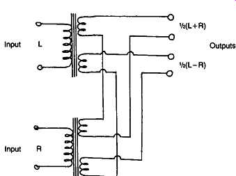
FIG. 10 Simple matrixing method.
The BBC system offers a CCIR weighted S/N ratio of 57 dB, and a non-linear distortion figure of 0.1% ref. full modulation at 1 kHz.
As in all digital systems, the prominence of the 'staircase type' step discontinuity becomes greater at low signal levels and higher audio frequencies, giving rise to a background noise associated with the signal, known as 'quantization noise'. Devotees of hi-fi tend to refer to these quantization effects as 'granularity'. Nevertheless, in spite of the relatively low standards, in the hi-fi context, adopted for the BBC PCM transmission links, there has been relatively little criticism of the sound quality of the broadcasts.
The encoding and decoding systems used are shown in Figs 11 and 12.
Encoding The operation of the PCM encoder, shown schematically in FIG. 11, may be explained by consideration of the operation of a single input channel. In this, the incoming signal is filtered, using a filter with a very steep attenuation rate, to remove all signal components above 15 kHz.
This is necessary since with a 32 kHz sampling rate, any audio components above half the sampling rate (say at 17 kHz) would be resolved identically to those at an equal frequency separation below this rate, (e.g. at 15 kHz), and this could cause severe problems both due to spurious signals, and to intermodulation effects between these signals. This problem is known as 'aliasing', and the filters are known as 'anti-aliasing' filters.
Because the quality of digitally encoded waveforms deteriorates as the signal amplitude gets smaller, it’s important to use the largest practicable signal levels (in which the staircase-type granularity will be as small a proportion of the signal as possible). It’s also important to ensure that the analogue-to-digital encoder is not overloaded. For this reason delay line type limiters are used, to delay the signal long enough for its amplitude to be assessed and appropriate amplitude limitation to be applied.
In order to avoid hard peak clipping which is audibly displeasing, the limiters operate by progressive reduction of the stage gain, and have an output limit of 4-2 dB above the nominal peak program level. Carrying out the limiting at this stage avoids the need for a further limiter at the transmitter. Pre-emphasis is also added before the limiter stage. The effect of this pre-emphasis on the frequency response is shown in FIG. 13.

FIG. 11 The BBC 13-channel pulse code modulation (PCM) encoder system.

FIG. 12 The BBC PCM decoding system.
An interesting feature of the limiter stages is that those for each stereo line pair are linked, so that if the peak level is exceeded on either, both channels are limited. This avoids any disturbance in stereo image location which might arise through a sudden amplitude difference between channels.
The AF bandwidth limited signal from the peak limiter is then converted into digital form by a clocked 'double ramp' analogue-to-digital converter, and fed, along with the bit streams from up to 12 other channels, to a time-domain multiplexing circuit. The output from this is fed through a filter, to limit the associated RF bandwidth, to an output line amplifier.
The output pulses are of sine-square form, with a half amplitude duration of 158 ns, and 158 ns apart. Since the main harmonic component of these pulses is the second, they have a negligible energy distribution above 6.336 MHz, which allows the complete composite digital signal to be handled by a channel designed to carry a 625-line TV program signal.
The output of the multiplexer is automatically sampled, sequentially, at 256 ms per program channel, in order to give an automatic warning of any system fault. It can also be monitored as an audio output signal reference.
To increase the immunity of the digitally encoded signal to noise or transmission line disturbances, a parity bit is added to each preceding 13 bit word. This contains data which provide an automatic check on the five most significant digits in the preceding bit group. If an error is detected, the faulty word is rejected and the preceding 13-bit word is substituted. If the error persists, the signal is muted until a satisfactory bit sequence is restored.
Effectively, therefore, each signal channel comprises 14 bits of information. With a sampling rate of 32 kHz, the 6.336 Mbits/s bandwidth allows a group of 198 bits in each sample period. This is built from 13 multiplexed 14-bit channels (= 182 bits) and 16 'spare' bits. Of these, 11 are used to control the multiplexing matrix, and four are used to carry transmitter remote control instructions.

FIG. 13 HF pre-emphasis characteristics.
Decoding:
The decoding system is shown in FIG. 12. In this the incoming bit stream is cleaned up, and restored to a sequence with definite __ and T states. The data stream is then used to regenerate the original 6336 kHz clock signal, and a counter system is used to provide a sequence of shift pulses fed, in turn, to 13 separate digital-to-analogue (D-A) converters, which recreate the original input channels, in analogue form.
A separate data decoder is used to extract the transmitter control information, and, as before, an automatic sampling monitor system is used to check the correct operation of each program channel.
The availability of spare channels can be employed to carry control information on a digitally controlled contrast compression/expansion (Compander) system (such as the BBC NIC AM 3 arrangement). This could be used either to improve the performance, in respect of the degradation of small signals, using the same number of sample steps, or to obtain a similar performance with a less good digital resolution (and less transmission bandwidth per channel). The standards employed for TV sound links, using a similar type of PCM studio-transmitter link, are:
• AF bandwidth, 50 Hz-13.5 kHz (± 0.7 dB 1 kHz)
• S/N ratio, 53 dB CCIR weighted
• non-linear distortion and quantization defects, 0.25% (ref. 1 kHz and max. modulation).
SUPPLEMENTARY BROADCAST SIGNALS
It has been suggested that data signals could be added to the FM or TV program signal, and this possibility is being explored by some European broadcasting authorities. The purpose of this would be to provide signal channel identification, and perhaps also to allow automatic channel tuning.
The system proposed for this would use an additional low level sub carrier , for example, at 57 kHz,. In certain regions of Germany additional transmissions based on this sub-carrier frequency are used to carry the VWF (road/traffic conditions) information broadcasts.
In the USA, 'Storecast' or 'Subsidiary Communication Authorization' (SCA) signals may be added to FM broadcasts, to provide a low-quality 'background music' program for subscribers to this scheme. This operates on a 67 kHz sub-carrier, with a max. modulation level of 10%.
ALTERNATIVE TRANSMISSION METHODS
Apart from the commercial (entertainment and news) broadcasts on the LW, MW and specified short wave bands shown in TBL. 2, where the transmission techniques are exclusively double-sideband amplitude modulated type, and in Band 2 (VHF) where the broadcasts are exclusively frequency modulated, there are certain police, taxi and other public utility broadcasts on Band 2 which are amplitude-modulated.
It’s planned that these other Band 2 broadcasts will eventually be moved to another part of the frequency spectrum, so that the whole of Band 2 can be available for FM radio transmissions.
However, there are also specific bands of frequencies, mainly in the HF/VHF parts of the spectrum, which have been allocated specifically for amateur use. These are shown in TBL. 3.
In these amateur bands, other types of transmitted signal modulation may be employed. These are narrow-bandwidth FM (NBFM), phase modulation (PM), and single-sideband suppressed carrier AM (SSB). The principal characteristics of these are that NBFM is restricted to a total deviation of ± 5 kHz, and a typical maximum modulation frequency of 3 kHz, limited by a steep-cut AF filter. This leads to a low modulation index (the ratio between the carrier deviation and the modulating frequency), which leads to poor audio quality and difficulties in reception (demodulation) without significant distortion. The typical (minimum) bandwidth requirement for NBFM is 13 kHz.
Phase modulation (PM), shares many of the characteristics of NBFM, except that in PM, the phase deviation of the signal is dependent both upon the amplitude and the frequency of the modulating signal, whereas in FM the deviation is purely dependent on program signal amplitude.
Both of these modulation techniques require fairly complex and well designed receivers, if good reception and S/N ratio is to be obtained.
TBL. 3 Amateur frequency band allocations
Band 80 M 40 M 20 M 15 M 10 M 6M 2 M MHz 3.5-3.725 7.0-7.15 14.0-14.35 21.0-21.45 28.0-29.7 50.0-54.0 144.0-148.0
SSB BROADCASTING
The final system, that of suppressed carrier single-sideband transmission (SSB), is very popular among the amateur radio transmitting fraternity, and will be found on all of the amateur bands.
This relies on the fact that the transmitted frequency spectrum of an AM carrier contains two identical, mirror-image, groups of sidebands below (lower sideband or LSB) and above (upper sideband or USB) the carrier, as shown in FIG. 14. The carrier itself conveys no signal and serves merely as the reference frequency for the sum and difference components which together reconstitute the original modulation.
If the receiver is designed so that a stable carrier frequency can be reintroduced, both the carrier and one of the sidebands can be removed entirely, without loss of signal intelligibility. This allows a very much larger proportion of the transmitter power to be used for conveying signal information, with a consequent improvement in range and intelligibility.
It also allows more signals to be accommodated within the restricted band
width allocation, and gives better results with highly selective radio receivers than would otherwise have been possible. The method employed is shown schematically in FIG. 15.

FIG. 14 Typical AM bandwidth spectrum for double-sideband transmission.

FIG. 15 Single sideband (USB or LSB) transmitter system.
There is a convention among amateurs that SSB transmissions up to 7 MHz shall employ LSB modulation, and those above this frequency shall use USB. This technique is not likely to be of interest to those concerned with good audio quality, but its adoption for MW radio broadcast reception is proposed from time to time, as a partial solution to the poor audio bandwidth possible with double sideband (DSB) transmission at contemporary 9 kHz carrier frequency separations.
The reason for this is that the DSB transmission system used at present only allows a 4.5 kHz AF bandwidth, whereas SSB would allow a full 9 kHz audio pass-band. On the other hand, even a small frequency drift of the reinserted carrier frequency can transpose all the program frequency components upwards or downwards by a step frequency interval, and this can make music sound quite awful; so any practical method would have to rely on the extraction and amplification of the residue of the original carrier, or on some equally reliable carrier frequency regeneration technique.
RADIO RECEIVER DESIGN
The basic requirements for a satisfactory radio receiver were listed above.
Although the relative importance of these qualities will vary somewhat from one type of receiver to another - say, as between an AM or an FM receiver - the preferred qualities of radio receivers are, in general, sufficiently similar for them to be considered as a whole, with some detail amendments to their specifications where system differences warrant this.

FIG. 16 Single (a) and bandpass (b) (c) tuned circuits.
Selectivity
An ideal selectivity pattern for a radio receiver would be one which had a constant high degree of sensitivity at the desired operating frequency, and at a sufficient bandwidth on either side of this to accommodate transmitter sidebands, but with zero sensitivity at all frequencies other than this.
A number of techniques have been used to try to approach this ideal performance characteristic. Of these, the most common is that based on the inductor-capacitor (LC) parallel tuned circuit illustrated in FIG. 16(a). Tuned circuit characteristics
For a given circulating RF current, induced into it from some external source, the AC potential appearing across an L-C tuned circuit reaches a peak value at a frequency (F0) given by the equation:
F0 = 1/(2 π √ LC)
Customarily the group of terms 2 pi F are lumped together and represented by the symbol ?, so that the peak output, or resonant frequency would be represented by:
ω0 = 1 / √LC
Inevitably there will be electrical energy losses within the tuned circuit, which will degrade its performance, and these are usually grouped together as a notional resistance, r, appearing in series with the coil.
The performance of such tuned circuits, at resonance, is quantified by reference to the circuit magnification factor or quality factor, referred to as Q. For any given L-C tuned circuit this can be calculated from Q = or - r ?0 0
Since, at resonance, the further equation can be derived. This shows that the Q improves as the equivalent loss resistance decreases, and as the ratio of L to C increases.
Typical tuned circuit Q values will lie between 50 and 200, unless the Q value has been deliberately degraded, in the interests of a wider RF signal pass-band, usually by the addition of a further resistor, R, in parallel with the tuned circuit.
The type of selectivity offered by such a single tuned circuit is shown , for various Q values, in FIG. 17(a). The actual discrimination against frequencies other than the desired one is clearly not very good, and can be calculated from the formula
σF = F0/2Q
where σ F is the 'half-power' bandwidth.
One of the snags with single tuned circuits, which is exaggerated if a number of such tuned circuits are arranged in cascade to improve the selectivity, is that the drop in output voltage from such a system, as the frequencies differ from that of resonance, causes a very rapid attenuation of higher audio frequencies in any AM type receiver, in which such a tuning arrangement was employed, as shown in curve 'a' of FIG. 18.
Clearly, this loss of higher audio frequencies is quite unacceptable, and the solution adopted for AM receivers is to use pairs of tuned circuits, coupled together by mutual inductance, Lm, or, in the case of separated circuits, by a coupling capacitor, Cc.

FIG. 17 Response curves of single (a) and bandpass (b) tuned circuits.

FIG. 18 Effect on AM receiver AF response of tuned circuit selectivity characteristics.
This leads to the type of flat-topped frequency response curve shown in FIG. 17(b), when critical coupling is employed, when the coupling factor For a mutually inductive coupled tuned circuit, this approximates to
Lm = L/Q
and for a capacitatively coupled bandpass tuned circuit.
Cc = C/Q
...where Lm is the required mutual inductance, L is the mean inductance of the coils, Ct is the mean value of the tuning capacitors, and Cc is the required coupling capacitance.
In the case of a critically-coupled bandpass tuned circuit, the selectivity is greater than that given by a single tuned circuit, in spite of the flat topped frequency response. Taking the case of F0 = 1 MHz, and Q = 100 , for both single- and double-tuned circuits the attenuation will be - 6 dB at 10 kHz off tune. At 20 kHz off tune, the attenuation will be -12 dB and -18 dB respectively, and at 30 kHz off tune it will be - 14 dB and -24 dB , for these two cases.
Because of the flat-topped frequency response possible with bandpass coupled circuits, it’s feasible to put these in cascade in a receiver design without incurring audio HF loss penalties at any point up to the beginning of the attenuation 'skirt' of the tuned circuit. For example, three such groups of 1 MHz bandpass-tuned circuits, with a circuit Q of 100, would give the following selectivity characteristics.
• 5 kHz = 0 dB
• 10 kHz = -18 dB
• 20 kHz = -54 dB
• 30 kHz = -72 dB
…as illustrated in curve 'b' in FIG. 18. Further, since the bandwidth is proportional to frequency, and inversely proportional to Q, the selectivity characteristics for any other frequency or Q value can be derived from these data by extrapolation.
Obviously this type of selectivity curve falls short of the ideal, especially in respect of the allowable audio bandwidth, but selectivity characteristics of this kind have been the mainstay of the bulk of AM radio receivers over the past sixty or more years. Indeed, because this represents an ideal case for an optimally designed and carefully aligned receiver, many commercial systems would be less good even than this.
For FM receivers, where a pass bandwidth of 220-250 kHz is required, only very low Q tuned circuits are usable, even at the 10.7 MHz frequency at which most of the RF amplification is obtained. So an alternative technique is employed, to provide at least part of the required adjacent channel selectivity. This is the surface acoustic wave filter.

FIG. 19 Construction of surface acoustic wave (SAW) filter.
The surface acoustic wave (SAW) filter
This device, illustrated in schematic form in FIG. 19, utilizes the fact that it’s possible to generate a mechanical wave pattern on the surface of a piece of piezo-electric material (one in which the mechanical dimensions will change under the influence of an applied electrostatic field), by applying an AC voltage between two electrically conductive strips laid on the surface of the material.
Since the converse effect also applies - that a voltage would be induced between these two conducting strips if a surface wave in a piezo-electric material were to pass under them - this provides a means for fabricating an electro-mechanical filter, whose characteristics can be tailored by the number, separation, and relative lengths of the conducting strips.
These SAW filters are often referred to as IDTs (inter-digital transducers), from the interlocking finger pattern of the metalizing, or simply as ceramic filters, since some of the earlier low-cost devices of this type were made from piezo-electric ceramics of the lead zirconate-titanate (PZT) type. Nowadays they are fabricated from thin, highly polished strips of lithium niobate, (LiNbO), bismuth germanium oxide, (BiGeO), or quartz on which a very precise pattern of metalizing has been applied by the same photo-lithographic techniques employed in the manufacture of integrated circuits.
Two basic types of SAW filter are used, of which the most common is the transversal type. Here a surface wave is launched along the surface from a transmitter group of digits to a receiver group. This kind is normally used for bandpass applications. The other form is the resonant type, in which the surface electrode pattern is employed to generate a standing-wave effect.
Because the typical propagation velocity of such surface waves is of the order of 3000 m/s, practical physical dimensions for the SAW slices and conductor patterns allow a useful frequency range without the need for excessive physical dimensions or impracticably precise electrode patterns.
Moreover, since the wave only penetrates a wavelength or so beneath the surface, the rear of the slice can be cemented onto a rigid substrate to improve the ruggedness of the element.
In the transversal or bandpass type of filter, the practicable range of operating frequencies is, at present, from a few MHz to 1-2 GHz, with minimum bandwidths of around 100 kHz. The resonant type of SAW device can operate from a few hundred kHz to a similar maximum frequency, and offers a useful alternative to the conventional quartz crystal (bulk resonator) for the higher part of the frequency range, where bulk resonator systems need to rely on oscillator overtones.
The type of performance characteristic offered by a bandpass SAW device, operating at a center frequency of 10.7 MHz, is shown in FIG. 20. An important quality of wide pass-band SAW filters is that the phase and attenuation characteristics can be separately optimized by manipulating the geometry of the pattern of the conducting elements deposited on the surface.
This is of great value in obtaining high audio quality from FM systems, as will be seen below, and differs, in this respect, from tuned circuits or other types of filter where the relative phase-angle of the transmitted signal is directly related to the rate of change of transmission as a function of frequency, in proximity to the frequency at which the relative phase angle is being measured.
However, there are snags. Good quality phase linear SAW filters are expensive, and there is a relatively high insertion loss, typically in the range of -15 to -25 dB, which requires additional compensatory amplification. On the other hand, they are physically small and don’t suffer, as do coils, from unwanted mutual induction effects. The characteristic impedance of such filters is, typically, 300-400 ohms, and changes in the source and load impedances can have big effects on the transmission curves.

FIG. 20 Transmission characteristics of typical 10.7 MHz SAW filter.