(adapted from Ben Duncan’s article in Stereophile, July 1995)
Have you ever suspected that the component you bought after diligent research is not "typical"? That its sound seems to bear little resemblance to the descriptions in the reviews you read? Sure, you listened to the unit before purchase, but the one you took out of the box at home--was that the same unit? And if you suspect your new unit's sonic quality is below par, just how do you or your dealer go about proving it? The inanimate world [1] created by mankind has as many foibles as the humans it delights in playing tricks on. Over a century ago, the English zoologist T.H. Huxley wrote, "The known is finite, the unknown infinite, intellectually we stand in an islet in … an illimitable ocean of inexplicability. Our business … is to reclaim a little more land." In this article, I will try to clear some of the mud off a few square yards -- homing in on the meaning of some manufacturing variations that occur in even the finest music-replay systems.
“IN A GOOD DESIGN, OVERALL TOLERANCES DO NOT DEPEND SO MUCH ON THE TOLERANCES OF THE INGREDIENTS.”
REAL-WORLD TOLERANCES
Like racing engines, the best hi-fi systems are finely tuned meaning the end result depends on many fine details. A small variation in just one of these details can cause an unexpectedly large loss of performance. Engines and sound systems are both built from many component parts, often thousands depending where you draw the line. Readers involved in any kind of engineering will be aware that every manufactured artifact differs slightly from the next. The range of differences between manufactured, ideally uniform objects is called tolerance. Awareness of tolerance—i.e., sameness--hinges on the ability to measure and resolve fine differences.
Metal can be cut, cast, or ground to tolerances of fractions of a millimeter--equivalent to tolerances better than, say, 0.01% for enclosures and heatsinks. Wood can't be measured meaningfully so finely, because it contracts and expands much more, and more readily, than metal, depending on temperature, humidity, and how long it has been seasoned. Capacitors and resistors-the wood and metal of electronics-are commonly made to comparatively loose tolerances of ± 1, 2,5, or 10%. Although the best equipment uses tighter resistor tolerances, up to 0.1%, capacitor tolerances tighter than 1% are rare and troublesome. The parameters of active devices (i.e., bipolar transistors, FETs, tubes, op-amps, and diodes) are held within ±5% at best and can be as broad as ± 70%, depending on cost, measurement temperature, design and manufacturing finesse, and the attribute in question. Transducer tolerances are as "loose" as active devices.
If an object has only one critical parameter (a measurable quality or attribute), then the manufacturer can simply decide on acceptable variation or difference, pick any samples that fall within this range, and reject any that don't. If 20% of the objects this test, then 80% will be rejects.
If more than one parameter is critical, and all have fairly poor tolerance the percentage of acceptable, usable production can drop drastically, perhaps to as low as 0.1%. In this case, we may have a badly designed, inefficient process. But if the rejects can be sold as "out-of-spec" (perhaps to the hobbyist market) used to make the “junior” version, or recycled, either internally or by other industries, then we have an “efficient”, “eco-friendly” process--but that's another story.
Demanding tolerances that are much more stringent than the natural spread of the manufacturing process greatly raises the cost of the components. Beyond a point, increasingly fine measurement, weighing adhesives (for toolmaking, casting, pressing, cutting wires, weighing adhesives, exposing films, measuring impedance, etc.) in the manufacture of raw materials and components, all the way up to finished gear, gets prohibitively expensive and time-consuming. Sources of error and "noise" multiply, and skilled human headwork is needed to extract meaningful data.
Traditionally, in a good design, overall tolerances do not depend so much on the tolerances of the ingredients. Engineers may use some kind of "sensitivity analysis" to assess and nurture this. A product that is acceptably precise yet can handle wide tolerance in its component parts (in electronics, negative feedback often facilitates this) is good for both ecology and profit.
The pragmatic manufacturer focuses on the (hopefully) small number of key parameters that have the most effect on the commercial product's conformity. The quality-conscious manufacturer aims to check the tolerances of the critical parts well before they are built into the product, as well as measuring critical parameters ("performance specs") after and sometimes during manufacture. This is called Quality Assurance, or QA. These letters may be writ large, but they form only a tiny part of the whole picture.
At this point it's worth noting that, whereas audio measurements cannot say anything specific about sonics (unless they show gross objective defects), an experienced test engineer often can correlate measurements for a specific design with that design's sonic qualities. He or she will quickly learn, for example, that a little kink (invisible to anew comer) in the distortion residue displayed on the oscilloscope means that the unit will sonically mis-perform in a particular way, and further, that this ties in with a particular part being defective.
In analog electronics, the problem of tolerance is quite different from that involved in, say, metalwork. In the latter, we are dealing with perhaps only two or three materials, and working in just three physical dimensions. Audio electronics is different, however, because the effects of departures from conformity are ultimately governed by psychoacoustics. This means that some aspects, like level—matching between an amplifier’s channels, can be quite loose; e.g., reasonable gain — matching between channels of ± 0.25dB corresponds to a tolerance of ± 3%, which is hardly demanding! Other aspects, like DAC linearity, have to be super-precise: to within a few parts per million, or in the region of 0.000001%.

Fig.1 Block schematic of the minimum disc replay path, used to analyze individual
systems’ frequency-response variations.
Electronic design usually involves large numbers of highly interdependent and mutually interactive parts, allowing an immense number of permutations. Intensifying the complexity is the fact that each type of component has more than one kind of tolerance. For example, the key parameter of a resistor is its resistance. By itself, this breaks down into several distinct tolerances. A resistor, say, measures 1000 ohms + T% at purchase, then + V% after W months storage, then + X% after soldering, and + Y% after Z thousand hours’ endurance in specified conditions of temperature and humidity.
This is bad enough. A resistor, however, is also affected by many other factors—temperature and voltage—resistance coefficients, shunt capacitance, series inductance, weldout crystallinity, and leadout purity—all of which will interact not only with each other, but, in even more complex ways, with all the other parts in the circuitry. The upshot is, if you look closely enough, the performance of the simplest circuit (one resistor draining a battery) is both individual and uniquely varies over time. With one component, the scale of the effect may be small enough to neglect. But what about the effects of the thousands of sound-influencing variables at large in even the simplest system?
THE TOLERANCE OF AMPLITUDE RESPONSE
To illustrate the effect of component tolerances on the simplest level, I entered a model of a minimal LP-replay system into MicroCAP, a PC-based circuit simulator. Looking at the block schematic (fig.1), the model comprises a cartridge (only the electrical internals are modeled), a cable, and a phono amp headed by a discrete buffer, followed by the RIAA EQ circuit, which uses two op-amps modeled on the ubiquitous NE5534 chip.
To simulate the effect of the RIAA pre-emphasis present on the disc, I have followed the preamp’s RIAA stage with a reference inverse RIAA circuit. (This was set to have perfect, zero tolerance in the simulation, so it plays no part in any variations.) There follows a volume control set 6dB below maximum, more cable, and a power amplifier with a typical voltage gain of x28, or just under 26dB. To make the simulation practicable, the last stage was simplified to be a power op-amp?
The full circuit contains a large number of parts, each with tolerances typical of mid- to high-end equipment, ranging from ± 1% for resistors, up to ± 60% for the looser active- device parameters (like Hfe, representing a transistor’s raw gain), and ±70% for cable parameters—allowing, within reason, for the different lengths used in real systems. As well as its value, in Ohms, Farads, or Henries, each passive component in the model has the tolerance of this quantity in ± % noted, and the temperature coefficient in ppm (parts per mil lion). Other than the simplifications noted, the model neglects long-term component value changes occurring over time, or one-off changes caused during manufacture by soldering and testing.
Fig.2 shows the frequency response, plotted from 1Hz to 100kHz, of this circuit, assuming zero, or perfect tolerance. On such a fine scale it isn’t perfectly flat, mirroring our many Audio Precision measurements of preamplifier disc (CD) inputs. Fig.3 shows 25 versions of the circuit’s response, the simulator progressively varying the tolerance of each part. The linear variation used is a halfway house between Gaussian, or “Normal” distribution (which doesn’t often happen in electronics manufacturing, apparently because some bigger, more macho customer, like Boeing, gets to pick out the best, “on-center” parts), and Worst Case distribution, which is overly pessimistic for a random equipment population. The Worst Case distribution, however, is good for setting production limits [ Note the fine vertical scale used in this graph, spanning just 1.25dB. This highlights the differences, which are of two kinds.
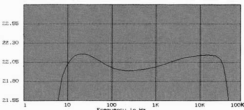
Fig.2 Predicted circuit frequency-response assuming zero tolerance (0.25dB/vertical
div.)
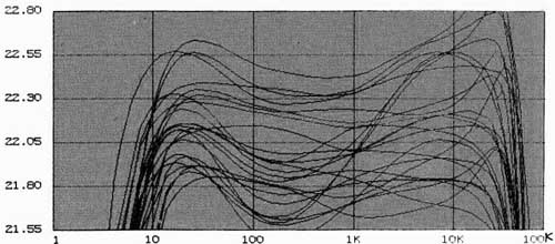
Fig.3 Predicted frequency-response variation in 25 randomly selected systems
(0.25dB/vertical div.).
First, the absolute level (or gain) varies by at least 1dB. This alone vindicates balance controls—even in the unlikely event that the loudspeakers are perfectly level—matched. More importantly, the variation in the population’s frequency response around the reference curve in fig.2 is complex. The biggest variation is at least ± 0.2dB, and some systems vary by more than ± 0.5dB. Although it may be hard to see, there are also one or two “golden” units that have a flatter, therefore more accurate response than the norm! Joe Smart always buys one of these, especially when the price has been knocked down to $50.
Fig.4 takes the scope of variability further into the real world by doubling all the close (below 10%) part tolerances to predict the effect of the gradual component value changes caused by long—term drift. These changes are accelerated by elevated operating and storage temperatures, and are caused by diffusion and electrophoresic effects; i.e., the migration of chemicals and ions under the prolonged influence of DC current flow. The variance picture is hard to see. MicroCAP’s statistical routines can output variance bar-chart data, but qualifying this is outside the scope of this piece; see [2]. But we can see that three distinct response—curve families have developed in fig.4 between 100Hz and 1kHz, and that the net variation is clearly wider. In turn, the graph’s span has been exactly doubled to 2.5dB to accommodate this.

Fig.4 Predicted lifetime frequency-response variation in 25 randomly selected
systems. Note that vertical scale is now doubled to 0.5dB/division. The variance
shown would be typical after several years’ use.

Fig.5 Typical variation in micro frequency response as the minimum disc replay
system warms up, from 20 to 70°C. The intermediate temperature of 45°C would
be more typical of “solid-states” equipment (0.25dB/vertical div.).
Fig.5 looks at a different kind of tolerance, the effect of the components’ temperature coefficients. These describe the rate of component value change with temperature. Again, the model is simplified, assuming a linear rate of change with temperature. This is true of good resistors [] over the likely temperatures endured by hi-fi equipment (generally 25- 85°C), but not perfectly true of most capacitors, excepting well-made polystyrene, polypropylene, and Teflon types [] Looking at the plots, the “micro” frequency response dearly varies as the equipment warms up—the LF response isn’t much changed, but the mid dips while the mild HF rise flat tens out. The difference between the “cold” and “operating- temperature” responses is an audible 0.25dB at 4kHz—this preamp will sound better as it “breaks in.”
Loudspeakers are even worse than electronic components when it comes to the effect of temperature. A loudspeaker’s voice-coil typically cycles between 20° and 200°C when driven by music. Its temperature coefficient is a huge 4000ppm/°C, meaning that its resistance nearly doubles over its operating range (i.e., increases by 100%, equivalent to 6dB of variance). The tuning of a typical passive crossover could be quite different at high power levels from what it was specified to be at a typical 1W level.
Altogether, these variations in frequency response are just a convenient abstract of the whole picture, which includes the spread of transient response (“speed” and “dynamics”), of linearity (i.e., distortion and the harmonic spectra, hence “timbre”; and intermodulation, hence “detail”), and of noise spectra (hence “ambience” and “depth”)—to mention just a few.
AT PRECISION’S EDGE
We know there are people who can clearly hear frequency- response differences of below 0.1dB [5]. Toward the low- and high-frequency extremes, where the unit-to-unit variability is most focused, the audibility of small differences will be exaggerated With reasonably neutral loudspeakers, the kind of variations illustrated will—when set against what balance and performance defects we are presently used to— determine whether we judge the system to be “bright” or “dull,” “articulate” or “authoritative:’ and so on. This applies less to owners than to reviewers, who have less time to strike up a relationship with a product.
A notable passage about audiophiles’ questing for the sonic grail comes from the “Letters” column of Electronics World A retired sound engineer wrote in 1986: “Ultimately, uncontrollable variations in manufacture result in what are, on a scale of perfection, gross differences between individual components So every unit will be slightly different.
But is this not true of all things in the universe? Excepting transient alignments, 100% conformity—with all the will and technology in the world—is bugged by the impossibility of 100% precision. In the real, competitive world, would-be king Conformity is cheated by people who pick out the best parts before the poor audio manufacturer gets to buy them, jostled by the random motion of molecules, undermined by the laws of entropy and chemical diffusion, then made uncertain by Quantum Mechanics. Finally, Conformity’s mental processes are thrown into a self-similar illogical chaos as number theory disintegrates at the portals of infinite numeric precision!
Ultimately, seeking precision willy-nilly is foolish; long before, it becomes explosively inefficient and expensive. To be realistic, we who care about fidelity in music reproduction can only concern ourselves with the scale of the variation and ask, on the basis of the latest psychoacoustic knowledge and listening experience, “Will it be enough to be audible— not just now, but maybe later?”
RAMIFICATIONS OF IMPERFECT SAMENESS
“They’ve all got better things to do / They may be false, they may be true / But nothing has been proved?’
The ramifications of tolerance concern everyone, but in different ways. As a QA-conscious manufacturer, I would have to pray that I was able to verify something the ear is quite fussy about by discovering the right objective test. Then I’d be worried about the extra cost of reworking units that filled the more exacting tests, and about the time taken to positively locate the part(s) causing the sonic variability. In the end, it comes down (in part) to employing sensitive humans who are able to couple their instinct and intuition to machines and objective knowledge Today, automated test equipment like the Audio Precision enables manufacturers to accumulate performance data, but very little of this is ever seen.
As a reviewer, I would be concerned about the single sample. If both channels sound (and continue to sound) the same, that’s a good start, and readers should be informed accordingly. To be sure, after getting used to the first sample, I would also like to hear at least three others, ideally with quite different serial numbers, or acquired randomly and incognito. In knowing the signature of the first unit, these would only require a brief listen by a well-endowed reviewer. The problem of progressive improvements made by the maker over time then arises. At the very least, I’d like to see some overlaid performance plots of a number of units, from the makers’ QA department, to see how much they vary.
As an owner, I might, depending on personal psychology, worry that the unit(s) I’d purchased weren’t typical or the best example In an existing system, if both channels sound about the same (e.g., listen in mono to each channel in turn), the main worry of a skewed stereo balance is cast aside. If not, untangling which units are causing the deviation, or which part of the deviation, is another story.
Before purchase, knowing about tolerance reinforces the need not just to listen yourself and preferably to “burn-in” components, but also to make sure that the unit you auditioned is the unit you take home Seeing how operating temperature influences performance suggests leaving equipment switched on as much as possible when you are the owner, but not before. Y’see, after learning that temperature cycling increases the rate at which initial component tolerances spread (compare fig.2 to the greater spread in flg.3), you will now ask the poor dealer to please cycle the power on/off for a week before you accept the home listening trial!
The designer’s challenge is not just to create stunning accuracy in reproduction, but also to have confidence in its repeatability and maintainability. In 1984, I wrote, “If we count the components inside each op-amp, there are around 350 in the signal path. . . and yet AMP-01 (an all-dancing, IC op-amp—based preamplifier) has so far out-maneuvered the folklore that the minimum number of parts is automatically the best, in the same way that a BMW overtakes a rickshaw on the road south from Kuala Lumpur?” [7] A valid reason for manufacturers using op-amp chips as the principal active devices in audio equipment is the consistency such devices promise Mere transistors, whether bipolar-junction transistors or FETs, are exceedingly complex devices, with more and more variable variables than the resistors, capacitors, and pots that surround them.
You may ask, if transistors are already complex, surely employing a complicated array of them in an IC just exacerbates the complexity? Well, first, IC design focuses on accepting large tolerance variations and on the special ability of monolithic parts to cancel out each other’s variations. Second, large amounts of negative feedback and a high gain-bandwidth-product together force uniformity. Third, the Central Limit Theorem of statistics predicts a counterintuitive concept: that complex systems can end up more predictable than simple ones.
Conversely, the equations used to generate fractal patterns bordering on chaos are simple ones; the “never-quite-the- same” complexity comes from partial positive feedback. Simple tube circuits with high impedance nodes are susceptible to inadvertent positive feedback, and, with messy wiring, can exhibit high variability in production. If both channels sound different, what good is the minimum signal path? But even small amounts of negative feedback— which can be intrinsic to even allegedly “feedback—free” topologies—are highly effective at limiting the degree to which hi-fi systems’ “tunings” can vary.
In my own designs I use not only precision, tightly QA’d op-amp ICs, but tighter—tolerance parts than the norm: I typically use 0.5 or 0.1% resistors with temperature coefficients of l5ppm, compared to hundreds of ppm for cheaper metal-film parts. But unless you make (or control the make up of) complete systems, this is gilding a lily with a growth on its leaves: the owner’s cable parameters, not to mention countless transducer tolerances, vary widely; worse, they’re outside the electronics designer’s control.
REFERENCES
Lyall Watson, The Nature of Things: The Secret Life of Inanimate Objects. Hodder & Stoughton, London, 1990.
R. Jeffs & D. Cook, “Generating Production Test Limits Based on Software-Derived Monte Carlo Analysis?” AES 11th International Conference, 1992.
Ben Duncan, “Pièce de Resistance, Part 2: Thermal Factors?” Hi-Pi News & Record Review, April 1987.
Ben Duncan, “With a Strange Device, Part 6: Temperature, Microphony, Tolerances & Reliability?’ Hi-Pi News & Record Review, November 1986.
Michael Gerzon, “Why Do Equalizers Sound Different?” Studio Sound, July 1990.
Roger Penrose, The Emperor’s New Mind: Concerning Computers, Minds and the Laws of Physics. Oxford University Press, 1989.
Ben Duncan, “AMP-Ol DIY Preamplifier?" Hi-Pi News & Record Review, September 1984.
== == ==
NOTES:
1. Before the advent of circuit simulation in the mid-’70s, tolerance analysis for any system containing hundreds of variables was too tedious to perform without teams of mathematicians, and not justifiable outside of critical space and military equipment. Instead, makers flew by the seats of their pants, and problems carried by out-of-tolerance (but in-spec) parts were usually only discovered by production tests or in the field, somewhat after the stable door had been bolted.
2. [MicroCAP] To save enough memory to make the simulation possible on a PC-XE the op-amp model behaves like an amplifier, but greatly reduces the number of nodes in the SPARSE matrix. The speaker cables’ and drive-unit’s electrical portions are excluded for the same reason. Even with all these simplifications, total parts count is around 200.
3. Leaving gear on, for example. If this alarms you, note that the alternative is worse, as switching components on and off is associated with temperature cycling, which accelerates time-to-death or catastrophic change.
4. Look at the Fletcher-Munson and related equal-loudness contour maps to see how the ear perceives a 4—5dB spl change as a doubling of loudness at 80Hz or 13kHz, compared to needing a 10dB change in spl at mid-frequencies.
5. Founded in 1912 as The Marconigraph, later Wireless World, Electronics World is the world’s oldest electronics journal, and has covered quality audio since the 1930s.
6. From “Scandal,” by Neil Tennant and Chris Lowe given urgency by Dusty Springfield in 1989.
== == ==
== ==
ALSO SEE:
== == ==