<< cont. from part 1
13. Burst correction
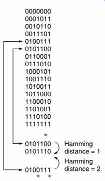
FIG. 18 All possible codewords of x^3 + x + 1 are shown, and the fact
that a double error in one codeword can produce the same pattern as a single
error in another. Thus double errors cannot be corrected.
FIG. 18 lists all the possible codewords in the code of FIG. 11.
Examination will show that it is necessary to change at least three bits in one codeword before it can be made into another. Thus the code has a Hamming distance of three and cannot detect three-bit errors. The single bit error correction limit can also be deduced from the figure. In the example given, the codeword 0101100 suffers a single-bit error marked * which converts it to a non-codeword at a Hamming distance of 1. No other codeword can be turned into this word by a single-bit error; therefore the codeword which is the shortest Hamming distance away must be the correct one. The code can thus reliably correct single-bit errors. However, the codeword 0100111 can be made into the same failure word by a two-bit error, also marked *, and in this case the original codeword cannot be found by selecting the one which is nearest in Hamming distance. A two-bit error cannot be corrected and the system will miscorrect if it is attempted.
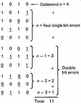
FIG. 19 Where double-bit errors occur, the number of patterns necessary
is (n - 1) + (n - 2) + (n - 3) + . . . Total necessary is 1 + n + (n -
1) + (n - 2) + (n - 3) + . . . etc.
Example here is of four bits, and all possible patterns up to a Hamming distance of two are shown (errors underlined).
The concept of Hamming distance can be extended to explain how more than one bit can be corrected. In FIG. 19 the example of two bits in error is given. If a codeword four bits long suffers a single-bit error, it could produce one of four different words. If it suffers a two-bit error, it could produce one of 3 + 2 + 1 different words as shown in the figure (the error bits are underlined). The total number of possible words of Hamming distance 1 or 2 from a four-bit codeword is thus:
4 + 3 + 2 + 1 = 10
If the two-bit error is to be correctable, no other codeword can be allowed to become one of this number of error patterns because of a two-bit error of its own. Thus every codeword requires space for itself plus all possible error patterns of Hamming distance 2 or 1, which is eleven patterns in this example. Clearly there are only sixteen patterns available in a four-bit code, and thus no data can be conveyed if two-bit protection is necessary.
The number of different patterns possible in a word of n bits is:
1 + n + (n-1) + (n-2) + (n-3) + . . .
and this pattern range has to be shared between the ranges of each codeword without overlap. For example, an eight-bit codeword could result in 1 + 8 + 7 + 6 + 5 + 4 + 3 + 2 + 1 = 37 patterns. As there are only 256 patterns in eight bits, it follows that only 256/37 pieces of information can be conveyed. The nearest integer below is six, and the nearest power of two below is four, which corresponds to two data bits and six check bits in the eight-bit word. The amount of redundancy necessary to correct any two bits in error is large, and as the number of bits to be corrected grows, the redundancy necessary becomes enormous and impractical. A further problem is that the more redundancy is added, the greater the probability of an error in a codeword. Fortunately, in practice errors occur in bursts, as has already been described, and it is a happy consequence that the number of patterns that result from the corruption of a codeword by adjacent two-bit errors is much smaller.
It can be deduced that the number of redundant bits necessary to correct a burst error is twice the number of bits in the burst for a perfect code. This is done by working out the number of received messages which could result from corruption of the codeword by bursts of from one bit up to the largest burst size allowed, and then making sure that there are enough redundant bits to allow that number of combinations in the received message.
Some codes, such as the Fire code due to Philip Fire, 4 are designed to correct single bursts, whereas later codes such as the B-adjacent code due to Bossen [5] could correct two bursts. The Reed-Solomon codes (Irving Reed and Gustave Solomon [6] ) have the advantage that an arbitrary number of bursts can be corrected by choosing the appropriate amount of redundancy at the design stage.
14. Introduction to the Reed-Solomon codes
The Reed-Solomon codes are inherently burst correcting because they work on multi-bit symbols rather than individual bits. The R-S codes are also extremely flexible in use. One code may be used both to detect and correct errors and the number of bursts which are correctable can be chosen at the design stage by the amount of redundancy. A further advantage of the R-S codes is that they can be used in conjunction with a separate error detection mechanism in which case they perform only the correction by erasure. R-S codes operate at the theoretical limit of correcting efficiency.
In other words, no more efficient code can be found.
In the simple CRC system described in sub-section 10, the effect of the error is detected by ensuring that the codeword can be divided by a polynomial.
The CRC codeword was created by adding a redundant symbol to the data.
In the Reed-Solomon codes, several errors can be isolated by ensuring that the codeword will divide by a number of polynomials. Clearly if the codeword must divide by, say, two polynomials, it must have two redundant symbols. This is the minimum case of an R-S code. On receiving an R-S coded message there will be two syndromes following the division. In the error-free case, these will both be zero. If both are not zero, there is an error.
It has been stated that the effect of an error is to add an error polynomial to the message polynomial. The number of terms in the error polynomial is the same as the number of errors in the codeword. The codeword divides to zero and the syndromes are a function of the error only. There are two syndromes and two equations. By solving these simultaneous equations it is possible to obtain two unknowns. One of these is the position of the error, known as the locator and the other is the error bit pattern, known as the corrector. As the locator is the same size as the code symbol, the length of the codeword is determined by the size of the symbol. A symbol size of eight bits is commonly used because it fits in conveniently with both sixteen-bit audio samples and byte-oriented computers. An eight-bit syndrome results in a locator of the same wordlength. Eight bits have 28 combinations, but one of these is the error-free condition, and so the locator can specify one of only 255 symbols. As each symbol contains eight bits, the codeword will be 255 _ 8 = 2040 bits long.
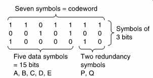
FIG. 20 A Reed-Solomon codeword. As the symbols are of three bits,
there can only be eight possible syndrome values. One of these is all zeros,
the error-free case, and so it is only possible to point to seven errors;
hence the codeword length of seven symbols. Two of these are redundant,
leaving five data symbols.
As further examples, five-bit symbols could be used to form a codeword 31 symbols long, and three-bit symbols would form a codeword seven symbols long. This latter size is small enough to permit some worked examples, and will be used further here. FIG. 20 shows that in the seven-symbol codeword, five symbols of three bits each, A-E, are the data, and P and Q are the two redundant symbols. This simple example will locate and correct a single symbol in error. It does not matter, however, how many bits in the symbol are in error.
The two check symbols are solutions to the following equations:
A _ B _ C _ D _ E _ P _ Q=0 [_ = XOR symbol] a^7 A _ a^6 B _ a^5 C _ a^4 D _ a^3 E _ a^2 P _ aQ=0
where a is a constant. The original data A-E followed by the redundancy P and Q pass through the channel.
The receiver makes two checks on the message to see if it is a codeword. This is done by calculating syndromes using the following expressions, where the () implies the received symbol which is not necessarily correct:
S0 =A _ B _ C _ D _ E _ P _ Q
(This is in fact a simple parity check)
S1= a^7 A _ a^6 B _ a^5 C _ a^4 D _ a^3 E _ a^2 P _ aQ
If two syndromes of all zeros are not obtained, there has been an error. The information carried in the syndromes will be used to correct the error. For the purpose of illustration, let it be considered that D has been corrupted before moving to the general case. D
can be considered to be the result of adding an error of value E to the original value D such that D = D _ E.
As A _ B _ C _ D _ E _ P _ Q=0 then A _ B _ C _ (D _ E) _ E _ P _ Q= E =S0
As D =D _ E then D = D _ E =D _ S0
Thus the value of the corrector is known immediately because it is the same as the parity syndrome S0. The corrected data symbol is obtained simply by adding S0 to the incorrect symbol.
At this stage, however, the corrupted symbol has not yet been identified, but this is equally straightforward:
As a^7 A _ a^6 B _ a^5 C _ a^4 D _ a^3 E _ a^2 P _ aQ=0
Then:
a^7 A _ a^6 B _ a^5 C _ a^4 (D _ E) _ a^3 E _ a^2 P _ aQ= a^4 E =S1
Thus the syndrome S1 is the error bit pattern E, but it has been raised to a power of a which is a function of the position of the error symbol in the block. If the position of the error is in symbol k, then k is the locator value and:
S0 _ ak =S1
Hence:
ak = S1 S0
The value of k can be found by multiplying S0 by various powers of a until the product is the same as S1. Then the power of a necessary is equal to k.
The use of the descending powers of a in the codeword calculation is now clear because the error is then multiplied by a different power of a dependent upon its position, known as the locator, because it gives the position of the error. The process of finding the error position by experiment is known as a Chien search. [7]
15. R-S Calculations
Whilst the expressions above show that the values of P and Q are such that the two syndrome expressions sum to zero, it is not yet clear how P and Q are calculated from the data. Expressions for P and Q can be found by solving the two R-S equations simultaneously. This has been done in Appendix 7.1. The following expressions must be used to calculate P and Q from the data in order to satisfy the codeword equations. These are:
P= a^6 A _ aB _ a^2 C _ a^5 D _ a^3 E
Q= a^2 A _ a^3 B _ a^6 C _ a^4 D _ aE
In both the calculation of the redundancy shown here and the calculation of the corrector and the locator it is necessary to perform numerous multiplications and raising to powers. This appears to present a formidable calculation problem at both the encoder and the decoder.
This would be the case if the calculations involved were conventionally executed. However, they can be simplified by using logarithms. Instead of multiplying two numbers, their logarithms are added. In order to find the cube of a number, its logarithm is added three times. Division is performed by subtracting the logarithms. Thus all the manipulations necessary can be achieved with addition or subtraction, which is straightforward in logic circuits.
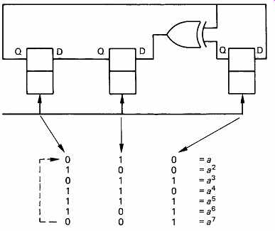
FIG. 21 The bit patterns of a Galois field expressed as powers of
the primitive element a. This diagram can be used as a form of log table
in order to multiply binary numbers. Instead of an actual multiplication,
the appropriate powers of a are simply added.
The success of this approach depends upon simple implementation of log tables. As was seen in Section 3, raising a constant, a, known as the primitive element, to successively higher powers in modulo 2 gives rise to a Galois field. Each element of the field represents a different power n of
a. It is a fundamental of the R-S codes that all the symbols used for data, redundancy and syndromes are considered to be elements of a Galois field. The number of bits in the symbol determines the size of the Galois field, and hence the number of symbols in the codeword.
FIG. 21 repeats a Galois field deduced in Section 3. The binary values of the elements are shown alongside the power of a they represent.
In the R-S codes, symbols are no longer considered simply as binary numbers, but also as equivalent powers of a. In Reed-Solomon coding and decoding, each symbol will be multiplied by some power of a. Thus if the symbol is also known as a power of a it is only necessary to add the two powers. For example, if it is necessary to multiply the data symbol 100 by a^3 , the calculation proceeds as follows, referring to FIG. 21:
100 = a^2 so 100 _ a^3 = a(2+3) = a^5 = 111
Note that the results of a Galois multiplication are quite different from binary multiplication. Because all products must be elements of the field, sums of powers which exceed seven wrap around by having seven subtracted. For example:
a^5 _ a^6 = a^11 = a^4 =110
FIG. 22 shows some examples of circuits which will perform this kind of multiplication. Note that they require a minimum amount of logic.
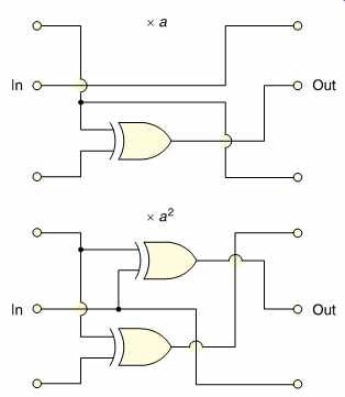
FIG. 22 Some examples of GF multiplier circuits.
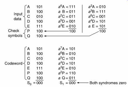
FIG. 23 Five data symbols A-E are used as terms in the generator polynomials
derived in Appendix 7.1 to calculate two redundant symbols P and Q. An
example is shown at the top. Below is the result of using the codeword
symbols A-Q as terms in the checking polynomials. As there is no error,
both syndromes are zero.
FIG. 23 shows an example of the Reed-Solomon encoding process.
The Galois field shown in FIG. 21 has been used, having the primitive element a = 010. At the beginning of the calculation of P, the symbol A is multiplied by a^6. This is done by converting A to a power of a. According to FIG. 21, 101 = a6 and so the product will be a (6+6) = a12 = a5 = 111.
In the same way, B is multiplied by a, and so on, and the products are added modulo-2. A similar process is used to calculate Q.
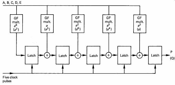
FIG. 24 If the five data symbols of FIG. 23 are supplied to this
circuit in sequence, after five clocks, one of the check symbols will appear
at the output. Terms without brackets will calculate P, bracketed terms
calculate Q.
FIG. 24 shows a circuit which can calculate P or Q. The symbols A-E are presented in succession, and the circuit is clocked for each one.
On the first clock, a^6 A is stored in the left-hand latch. If B is now provided at the input, the second GF multiplier produces aB and this is added to the output of the first latch and when clocked will be stored in the second latch which now contains a^6 A + aB. The process continues in this fashion until the complete expression for P is available in the right hand latch. The intermediate contents of the right-hand latch are ignored.
The entire codeword now exists, and can be recorded or transmitted.
FIG. 23 also demonstrates that the codeword satisfies the checking equations. The modulo 2 sum of the seven symbols, S0, is 000 because each column has an even number of ones. The calculation of S1 requires multiplication by descending powers of a. The modulo-2 sum of the products is again zero. These calculations confirm that the redundancy calculation was properly carried out.
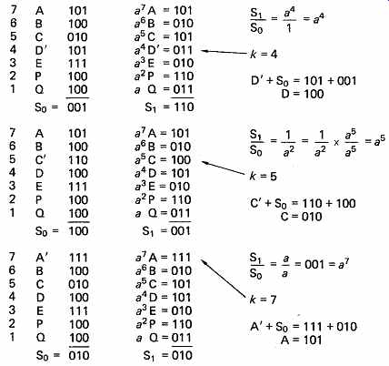
FIG. 25 Three examples of error location and correction. The number
of bits in error in a symbol is irrelevant; if all three were wrong, S0
would be 111, but correction is still possible.
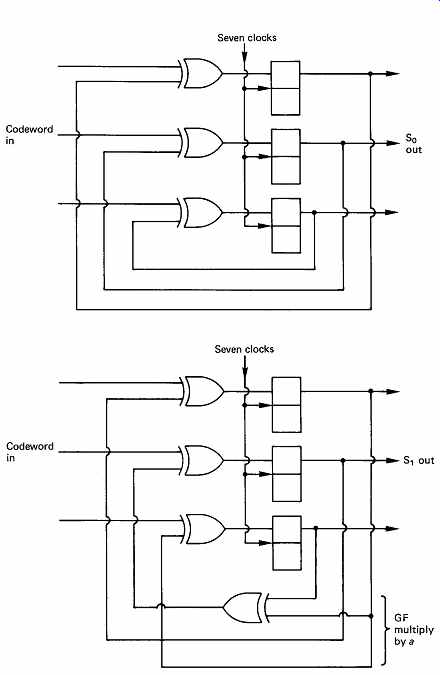
FIG. 26 Circuits for parallel calculation of syndromes S0, S1. S0
is a simple parity check. S1 has a GF multiplication by a in the feedback,
so that A is multiplied by a^7 , B is multiplied by a^6 , etc., and all
are summed to give S1.
FIG. 25 gives three examples of error correction based on this codeword. The erroneous symbol is marked with a dash. As there has been an error, the syndromes S0 and S1 will not be zero.
FIG. 26 shows circuits suitable for parallel calculation of the two syndromes at the receiver. The S0 circuit is a simple parity checker which accumulates the modulo-2 sum of all symbols fed to it. The S1 circuit is more subtle, because it contains a Galois field (GF) multiplier in a feedback loop, such that early symbols fed in are raised to higher powers
than later symbols because they have been recirculated through the GF multiplier more often. It is possible to compare the operation of these circuits with the example of FIG. 25 and with subsequent examples to confirm that the same results are obtained.
16. Correction by erasure
In the examples of FIG. 25, two redundant symbols P and Q have been used to locate and correct one error symbol. If the positions of errors are known by some separate mechanism (see product codes, section 7.18) the locator need not be calculated. The simultaneous equations may instead be solved for two correctors. In this case the number of symbols which can be corrected is equal to the number of redundant symbols. In FIG. 27(a) two errors have taken place, and it is known that they are in symbols C and D. Since S0 is a simple parity check, it will reflect the modulo-2 sum of the two errors. Hence S0 = EC _ ED.
The two errors will have been multiplied by different powers in S1, such that:
S1 = a^5 EC _ a^4 ED
These two equations can be solved, as shown in the figure, to find EC and ED, and the correct value of the symbols will be obtained by adding these correctors to the erroneous values. It is, however, easier to set the values of the symbols in error to zero. In this way the nature of the error is rendered irrelevant and it does not enter the calculation. This setting of symbols to zero gives rise to the term erasure. In this case,
S0 =C _ D
S1 = a^5 C _ a^4 D
Erasing the symbols in error makes the errors equal to the correct symbol values and these are found more simply as shown in FIG. 27(b).
Practical systems will be designed to correct more symbols in error than in the simple examples given here. If it is proposed to correct by erasure an arbitrary number of symbols in error given by t, the codeword must be divisible by t different polynomials. Alternatively if the errors must be located and corrected, 2t polynomials will be needed. These will be of the form (x + an) where n takes all values up to t or 2t. a is the primitive element discussed in Section 3.
Where four symbols are to be corrected by erasure, or two symbols are to be located and corrected, four redundant symbols are necessary, and the codeword polynomial must then be divisible by
(x + a0 )(x + a1)(x + a2)(x + a3)
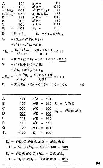

FIG. 27 If the location of errors is known, then the syndromes are
a known function of the two errors as shown in (a). It is, however, much
simpler to set the incorrect symbols to zero, i.e. to erase them as in
(b). Then the syndromes are a function of the wanted symbols and correction
is easier.
Upon receipt of the message, four syndromes must be calculated, and the four correctors or the two error patterns and their positions are determined by solving four simultaneous equations. This generally requires an iterative procedure, and a number of algorithms have been developed for the purpose. [8-10]
Modern digital audio formats such as CD and DAT use eight-bit R-S codes and erasure extensively. The primitive polynomial commonly used with GF(256) is x^8 + x^4 + x^3 + x^2 + 1
The codeword will be 255 bytes long but will often be shortened by puncturing. The larger Galois fields require less redundancy, but the computational problem increases. LSI chips have been developed specifically for R-S decoding in many high-volume formats. [11,12]
As an alternative to dedicated circuitry, it is also possible to perform Reed- Solomon calculations in software using general-purpose processors.[13] This may be more economical in small-volume products.
17. Interleaving
The concept of bit interleaving was introduced in connection with a single bit correcting code to allow it to correct small bursts. With burst-correcting codes such as Reed-Solomon, bit interleave is unnecessary. In most channels, particularly high-density recording channels used for digital audio, the burst size may be many bytes rather than bits, and to rely on a code alone to correct such errors would require a lot of redundancy. The solution in this case is to employ symbol interleaving, as shown in FIG. 28. Several codewords are encoded from input data, but these are not recorded in the order they were input, but are physically reordered in the channel, so that a real burst error is split into smaller bursts in several codewords. The size of the burst seen by each codeword is now determined primarily by the parameters of the interleave, and FIG. 29 shows that the probability of occurrence of bursts with respect to the burst length in a given codeword is modified. The number of bits in the interleave word can be made equal to the burst-correcting ability of the code in the knowledge that it will be exceeded only very infrequently.
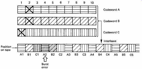
FIG. 28 The interleave controls the size of burst errors in individual
codewords.
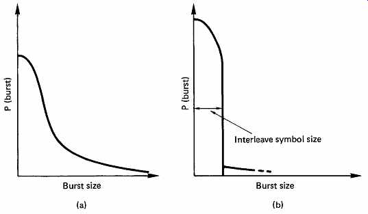
FIG. 29 (a) The distribution of burst sizes might look like this.
(b) Following interleave, the burst size within a codeword is controlled
to that of the interleave symbol size, except for gross errors which have
low probability.
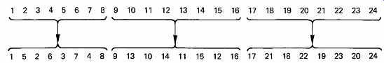
FIG. 30 In block interleaving, data are scrambled within blocks which
are themselves in the correct order.
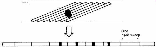
FIG. 31 Helical-scan recorders produce a form of mechanical interleaving,
because one large defect on the medium becomes distributed over several
head sweeps.
There are a number of different ways in which interleaving can be performed. FIG. 30 shows that in block interleaving, words are reordered within blocks which are themselves in the correct order. This approach is attractive for rotary-head recorders, such as DAT, because the scanning process naturally divides the tape up into blocks. The block interleave is achieved by writing samples into a memory in sequential address locations from a counter, and reading the memory with non sequential addresses from a sequencer. The effect is to convert a one dimensional sequence of samples into a two-dimensional structure having rows and columns.
Rotary-head recorders naturally interleave spatially on the tape. FIG. 31 shows that a single large tape defect becomes a series of small defects owing to the geometry of helical scanning.
The alternative to block interleaving is convolutional interleaving where the interleave process is endless. In FIG. 32 symbols are assembled into short blocks and then delayed by an amount proportional to the position in the block. It will be seen from the figure that the delays have the effect of shearing the symbols so that columns on the left side of the diagram become diagonals on the right. When the columns on the right are read, the convolutional interleave will be obtained. Convolutional interleave works well with stationary head recorders where there is no natural track break and with CD where the track is a continuous spiral.
Convolutional interleave has the advantage of requiring less memory to implement than a block code. This is because a block code requires the entire block to be written into the memory before it can be read, whereas a convolutional code requires only enough memory to cause the required delays. Now that RAM is relatively inexpensive, convolutional interleave is less popular.
It is possible to make a convolutional code of finite size by making a loop. FIG. 33(a) shows that symbols are written in columns on the outside of a cylinder. The cylinder is then sheared or twisted, and the columns are read. The result is a block-completed convolutional interleave shown at (b). This technique is used in the digital audio blocks of the Video-8 format.
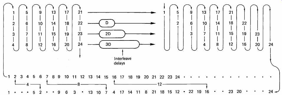
FIG. 32 In convolutional interleaving, samples are formed into a rectangular
array, which is sheared by subjecting each row to a different delay. The
sheared array is read in vertical columns to provide the interleaved output.
In this example, samples will be found at 4, 8 and 12 places away from
their original order.
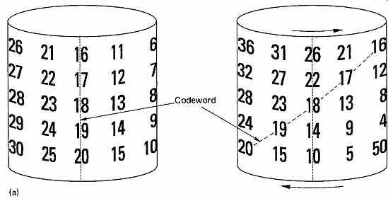
FIG. 33 (a) A block-completed convolutional interleave can be considered
to be the result of shearing a cylinder.
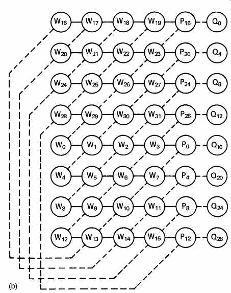
FIG. 33 (b) A block completed convolutional interleave results in
horizontal and diagonal codewords as shown here.
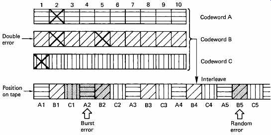
FIG. 34 The interleave system falls down when a random error occurs
adjacent to a burst.
18. Product codes
In the presence of burst errors alone, the system of interleaving works very well, but it is known that in most practical channels there are also uncorrelated errors of a few bits due to noise. FIG. 34 shows an interleaving system where a dropout-induced burst error has occurred which is at the maximum correctable size. All three codewords involved are working at their limit of one symbol. A random error due to noise in the vicinity of a burst error will cause the correction power of the code to be exceeded. Thus a random error of a single bit causes a further entire symbol to fail. This is a weakness of an interleave solely designed to handle dropout-induced bursts. Practical high-density equipment must address the problem of noise-induced or random errors and burst errors occurring at the same time. This is done by forming codewords both before and after the interleave process. In block interleaving, this results in a product code, whereas in the case of convolutional interleave the result is called cross-interleaving. [14]
FIG. 35 shows that in a product code the redundancy calculated first and checked last is called the outer code, and the redundancy calculated second and checked first is called the inner code. The inner code is formed along tracks on the medium. Random errors due to noise are corrected by the inner code and do not impair the burst-correcting power of the outer code. Burst errors are declared uncorrectable by the inner code which flags the bad samples on the way into the de-interleave memory. The outer code reads the error flags in order to correct the flagged symbols by erasure. The error flags are also known as erasure flags. As it does not have to compute the error locations, the outer code needs half as much redundancy for the same correction power. Thus the inner code redundancy does not raise the code overhead. The combination of codewords with interleaving in several dimensions yields an error-protection strategy which is truly synergistic, in that the end result is more powerful than the sum of the parts. Needless to say, the technique is used extensively in modern formats such DAT and DCC. The error correction strategy of DAT is treated in the next section as a representative example of a modern product code.
An alternative to the product block code is the convolutional cross interleave, shown in FIG. 32. In this system, the data are formed into an endless array and the codewords are produced on columns and diagonals. The Compact Disc and DASH formats use such a system. The original advantage of the cross-interleave is that it needed less memory than a product code. This advantage is no longer so significant now that memory prices have fallen so much. It has the disadvantage that editing is more complicated. The error-correction system of CD is discussed in detail in Section 12.
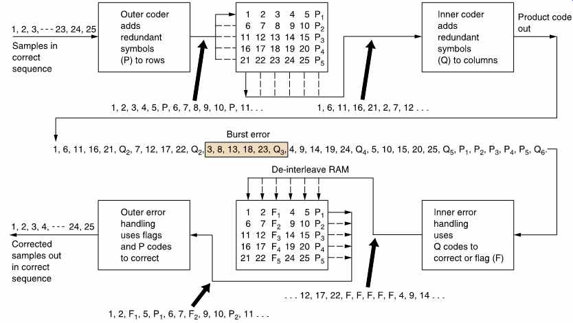
FIG. 35 In addition to the redundancy P on rows, inner redundancy
Q is also generated on columns. On replay, the Q code checker will pass
on flags F if it finds an error too large to handle itself. The flags pass
through the de-interleave process and are used by the outer error correction
to identify which symbol in the row needs correcting with P redundancy.
The concept of crossing two codes in this way is called a product code.
19. Introduction to error correction in DAT
The interleave and error-correction systems of DAT will now be discussed. FIG. 36 is a conceptual block diagram of the system which shows that DAT uses a product code formed by producing Reed- Solomon codewords at right angles across an array. The array is formed in a memory, and the layout used in the case of 48 kHz sampling can be seen in FIG. 37.
There are two recorded tracks for each drum revolution and incoming samples for that period of time are routed to a pair of memory areas of 4 bytes capacity, one for each track. These memories are structured as 128 columns of 32 bytes each. The error correction works with eight-bit symbols, and so each sample is divided into high byte and low byte and occupies two locations in memory. FIG. 37 shows only one of the two memories. Incoming samples are written across the memory in rows, with the exception of an area in the center, 24 bytes wide. Each row of data in the RAM is used as the input to the Reed- Solomon encoder for the outer code. The encoder starts at the left-hand column, and then takes a byte from every fourth column, finishing at column 124 with a total of 26 bytes. Six bytes of redundancy are calculated to make a 32 byte outer codeword. The redundant bytes are placed at the top of columns 52, 56, 60, etc. The encoder then makes a second pass through the memory, starting in the second column and taking a byte from every fourth column finishing at column 125. A further six bytes of redundancy are calculated and put into the top of columns 53, 57, 61, and so on. This process is performed four times for each row in the memory, except for the last eight rows where only two passes are necessary because odd-numbered columns have sample bytes only down to row 23. The total number of outer codewords produced is 112.
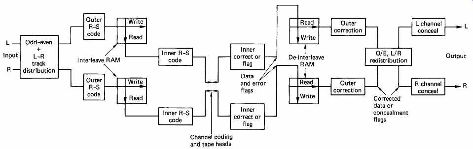
FIG. 36 The error-protection strategy of DAT. To allow concealment
on replay, an odd/even, left/right track distribution is used. Outer codes
are generated on RAM rows, inner codes on columns. On replay, inner codes
correct random errors. Flags pass through de-interleave RAM to outer codes
which use them as erasure pointers. Uncorrected errors can be concealed
after redistribution to real-time sequence.
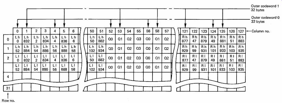
FIG. 37 Left even/right odd interleave memory. Incoming samples are
split into high byte (h) and low byte (l), and written across the memory
rows using first the even columns for L 0-830 and R 1-831, and then the
odd columns for L 832-1438 and R 833-1439. For 44.1 kHz working, the number
of samples is reduced from 1440 to 1323, and fewer locations are filled.
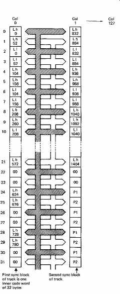
FIG. 38 The columns of memory are read out to form inner codewords.
First, even bytes from the first two columns make one codeword and then
odd bytes from the first two columns. As there are 128 columns, there will
be 128 sync blocks in one audio segment.
In order to encode the inner codewords to be recorded, the memory is read in columns. FIG. 38 shows that, starting at top left, bytes from the sixteen even-numbered rows of the first column, and from the first twelve even-numbered rows of the second column, are assembled and fed to the inner encoder. This produces four bytes of redundancy which are written into the memory in the areas marked P1. Four bytes P1, when added to the 28 bytes of data, makes an inner codeword 32 bytes long. The second inner code is encoded by making a second pass through the first two columns of the memory to read the samples on odd-numbered rows. Four bytes of redundancy are placed in memory in locations marked P2. Each column of memory is then read completely and becomes one sync block on tape. Two sync blocks contain two interleaved inner codes such that the inner redundancy for both is at the end of the second sync block. The effect is that adjacent symbols in a sync block are not in the same codeword. The process then repeats down the next two columns in the memory and so on until 128 blocks have been written to the tape.
Upon replay, the sync blocks will suffer from a combination of random errors and burst errors. The effect of interleaving is that the burst errors will be converted to many single-symbol errors in different outer codewords.
As there are four bytes of redundancy in each inner codeword, a theoretical maximum of two bytes can be corrected. The probability of miscorrection in the inner code is minute for a single-byte error, because all four syndromes will agree on the nature of the error, but the probability of miscorrection on a double-byte error is much higher. The inner code logic is exposed to random noise during dropout and mistracking conditions, and the probability of noise producing what appears to be only a two-symbol error is too great. If more than one byte is in error in an inner code it is more reliable to declare all bytes bad by attaching flags to them as they enter the de-interleave memory. The interleave of the inner codes over two sync blocks is necessary because of the use of a group code. In the 8/10 code described in Section 6, a single mispositioned transition will change one ten-bit group into another, potentially corrupting up to eight data bits. A small disturbance at the boundary between two groups could corrupt up to sixteen bits. By interleaving the inner codes at symbol level, the worst case of a disturbance at the boundary of two groups is to produce a single-symbol error in two different inner codes. Without the inner code interleave, the entire contents of an inner code could be caused to be flagged bad by a single small defect. The inner code interleave halves the error propagation of the group code, which increases the chances of random errors being corrected by the inner codes instead of impairing the burst-error correction of the outer codes.
After de-interleave, any uncorrectable inner codewords will show up as single-byte errors in many different outer codewords accompanied by error flags. To guard against miscorrections in the inner code, the outer code will calculate syndromes even if no error flags are received from the inner code. If two bytes or less in error are detected, the outer code will correct them even though they were due to inner code miscorrections.
This can be done with high reliability because the outer code has three byte detecting and correcting power which is never used to the full. If more than two bytes are in error in the outer codeword, the correction process uses the error flags from the inner code to correct up to six bytes in error.
The reasons behind the complex interleaving process now become clearer. Because of the four-way interleave of the outer code, four entire sync blocks can be destroyed, but only one byte will be corrupted in a given outer codeword. As an outer codeword can correct up to six bytes in error by erasure, it follows that a burst error of up to 24 sync blocks could be corrected. This corresponds to a length of track of just over 2.5mm, and is more than enough to cover the tenting effect due to a particle of debris lifting the tape away from the head. In practice the interleave process is a little more complicated than this description would suggest, owing to the requirement to produce recognizable sound in shuttle. This process will be detailed in Section 9.
20. Editing interleaved recordings
The interleave, de-interleave, time-compression and timebase-correction processes cause delay and this is evident in the time taken before audio emerges after starting a digital machine. Confidence replay takes place later than the distance between record and replay heads would indicate.
In DASH format recorders, confidence replay is about one tenth of a second behind the input. Processes such as editing and synchronous recording require new techniques to overcome the effect of the delays.
In analog recording, there is a direct relationship between the distance down the track and the time through the recording and it is possible to mark and cut the tape at a particular time. A further consequence of interleaving in digital recorders is that the reordering of samples means that this relationship is lost.
Editing must be undertaken with care. In a block-based interleave, edits can be made at block boundaries so that coded blocks are not damaged, but these blocks are usually too large for accurate audio editing. In a convolutional interleave, there are no blocks and an edit or splice will damage diagonal codewords over a constraint length near the edit as shown in FIG. 39.
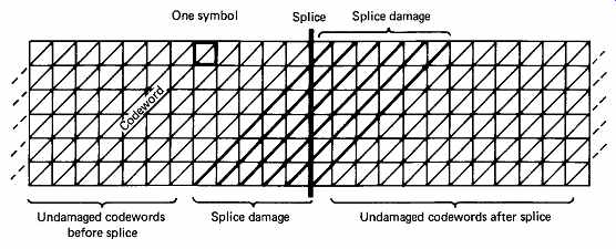
FIG. 39 Although interleave is a powerful weapon against burst errors,
it causes greater data loss when tape is spliced because many codewords
are replayed in two unrelated halves.

FIG. 40 In the most sophisticated version of audio editing, there
are advanced replay heads on the scanner, which allow editing to be performed
on de-interleaved data. An insert sequence is shown. In (a) the replay-head
signal is decoded and fed to the encoder which, after some time, will produce
an output representing what is already on the tape. In (b), at a sector
boundary, the write circuits are turned on, and the machine begins to re-record.
In (c) the crossfade is made to the insert material. In (d) the insert
ends with a crossfade back to the signal from the advanced replay heads.
After this, the write heads will once again be recording what is already
on the tape, and the write circuits can be disabled at a sector boundary.
An assemble edit consists of the first three of these steps only.
The only way in which audio can be edited satisfactorily in the presence of interleave is to use a read-modify-write approach, where an entire frame is read into memory and de-interleaved to the real-time sample sequence. Any desired part of the frame can be replaced with new material before it is re-interleaved and re-recorded. In recorders which can only record or play at one time, an edit of this kind would take a long time because of all the tape repositioning needed. With extra heads read-modify-write editing can be performed dynamically.
The sequence is shown in FIG. 40 for a rotary-head machine but is equally applicable to stationary head transports. The replay head plays back the existing recording, and this is de-interleaved to the normal sample sequence, a process which introduces a delay. The sample stream now passes through a crossfader which at this stage will be set to accept only the offtape signal. The output of the crossfader is then fed to the record interleave stage which introduces further delay. This signal passes to the record heads which must be positioned so that the original recording on the tape reaches them at the same time that the re-encoded signal arrives, despite the encode and decode delays. In a rotary-head recorder this can be done by positioning the record heads at a different height to the replay heads so that they reach the same tracks on different revolutions. With this arrangement it is possible to enable the record heads at the beginning of a frame, and they will then re-record what is already on the tape. Next, the crossfader can be operated to fade across to new material, at any desired crossfade speed. Following the interleave stage, the new recording will update only the new samples in the frame and re-record those which do not need changing. After a short time, the recording will only be a function of the new input. If the edit is an insert, it is possible to end the process by crossfading back to the replay signal and allowing the replay data to be re-recorded. Once this re-recording has taken place for a short time, the record process can be terminated at the end of a frame. There is no limit to the crossfade periods which can be employed in this operating technique, in fact the crossfade can be manually operated so that it can be halted at a suitable point to allow, for example, a commentary to be superimposed upon a recording.
One important point to appreciate about read-modify-write editing is that the physical frames at which the insert begins and ends are independent of the in- and out-points of the audio edit, because the former are in areas where re-recording of the existing data takes place.
Electronic editing and tape-cut editing of digital recordings is discussed in Section 11.
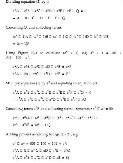
Appendix 1: Calculation of Reed-Solomon generator polynomials
For a Reed-Solomon codeword over GF(23 ), there will be seven three-bit symbols. For location and correction of one symbol, there must be two redundant symbols P and Q, leaving A-E for data.
The following expressions must be true, where a is the primitive element of x^3 _ x _ 1 and _ is XOR throughout:
A _ B _ C _ D _ E _ P _ Q=0 (1)
a^7 A _ a^6 B _ a^5 C _ a^4 D _ a^3 E _ a^2 P _ aQ=0 (2)
References
1. Michaels, S.R., Is it Gaussian? Electronics World and Wireless World, 72-73 (January 1993)
2. Shannon, C.E., A mathematical theory of communication. Bell System Tech. J., 27, 379 (1948)
3. Hamming, R.W., Error-detecting and error-correcting codes. Bell System Tech. J., 26, 147-160 (1950)
4. Fire, P., A class of multiple-error correcting codes for non-independent errors. Sylvania Reconnaissance Systems Lab. Report, RSL-E-2 (1959)
5. Bossen, D.C., B-adjacent error correction. IBM J. Res. Dev., 14, 402-408 (1970)
6. Reed, I.S. and Solomon, G., Polynomial codes over certain finite fields. J. Soc. Indust. Appl. Math., 8, 300-304 (1960)
7. Chien, R.T., Cunningham, B.D. and Oldham, I.B., Hybrid methods for finding roots of a polynomial - with application to BCH decoding. IEEE Trans. Inf. Theory., IT-15, 329-334 (1969)
8. Berlekamp, E.R., Algebraic Coding Theory, New York: McGraw-Hill (1967). Reprint edition: Laguna Hills, CA: Aegean Park Press (1983)
9. Sugiyama, Y. et al., An erasures and errors decoding algorithm for Goppa codes. IEEE Trans. Inf. Theory, IT-22 (1976)
10. Peterson, W.W. and Weldon, E.J., Error Correcting Codes, 2nd edn., Cambridge, MA: MIT Press (1972)
11. Onishi, K., Sugiyama, K., Ishida, Y., Kusonoki, Y. and Yamaguchi, T., An LSI for Reed- Solomon encoder/decoder. Presented at the 80th Audio Engineering Society Convention (Montreux, 1986), Preprint 2316(A-4)
12. Anon. Digital Audio Tape Deck Operation Manual, Sony Corporation (1987)
13. van Kommer, R., Reed-Solomon coding and decoding by digital signal processors. Presented at the 84th Audio Engineering Society Convention ( Paris, 1988), Preprint 2587(D-7)
14. Doi, T.T., Odaka, K., Fukuda, G. and Furukawa, S. Cross-interleave code for error correction of digital audio systems. J. Audio Eng. Soc., 27, 1028 (1979)
===