In the acoustics field, white noise sources are frequently employed along with octave and one-third octave band filters. Typical applications include the measurement of transducer characteristics, material absorption-reflection and transmission coefficients, and room parameters such as reverberation time. One problem commonly encountered in making these measurements is that the noise signal detected falls off greatly at low frequencies since the rms noise passed by the filter varies as the square root of the filter bandwidth, and hence the center frequency of the filter.
Generally one compensates for this effect lay increasing the power-amplifier gain when the lower frequencies are to be examined; but, since the filter is usually connected at the output (Fig. 1), this increased gain can result in an overload of both the power amplifier and the loudspeaker.
A more practical solution to this problem is to convert the random noise source from one having a constant energy/cycle, or white noise frequency spectrum, to a constant energy/octave, or pink noise response. This may be accomplished by employing a conventional white noise source and connecting a "pink noise filter" to its output. This type of filter basically has a transmission characteristic which falls off inversely as the square root of the applied frequency (Fig. 5). The rms output from such a pink noise source will then be independent of the octave band being examined (Fig. 2). A simple circuit for achieving this type of filtering in the audio range from 10 hz to 20 khz is shown in Fig. 3, with the general form of one of the stages given in Fig. 4.
Since d.c. coupling of the stages is employed, Rb is set equal to zero to minimize the d.c. gain of each stage, and hence the effect of d.c. offset voltages on filter stability. Using Fig. 5 as a guide, a-20 dB/decade piecewise approximation is employed using three stages with their break frequencies selected to provide the best possible fit to the -10 dB/decade desired slope. This requires three curves of the type shown in Fig. 4, spaced a decade apart in frequency, and allows for the use of the same resistors in each stage by simply changing the capacitor by a power of 10 to shift the breakpoints to the desired location. The addition of the RC break frequency at f1 = 17.78 kHz at the input of IC3 extends the accuracy of the response to beyond 30 kHz.
It should be noted that when using the filter there is no impedance matching problem since its frequency characteristics are essentially independent of the source and load impedances connected to it; in addition, any available supply voltages from ±6 to ±18 volts can be utilized. If 1 percent resistors and 5 percent capacitors are employed, the response should be accurate to within one dB of the desired characteristic.
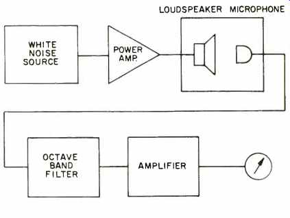
Fig. 1-General measurement technique.
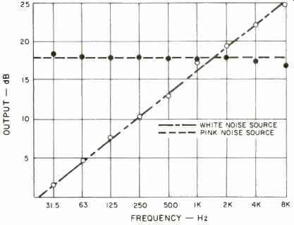
Fig. 2-Actual noise source outputs vs. frequency when examined in octave
bands.
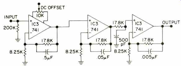
Fig. 3-Audio pink noise filter design.
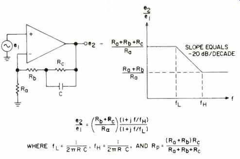
Fig. 4-Single stage characteristic.
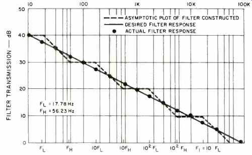
Fig. 5-Actual filter transmission characteristic.
(Source: Audio magazine, March 1977; Dr. Robert Mauro [Assistant Professor of Electrical Engineering, Manhattan College, Riverdale, N.Y.])
= = = =