|
|
Malcolm Hawksford had his first design, a console tape recorder with pre- and power amp and build-in loudspeakers, published in the prestigious Hi-Fi News in June 1963 at age 5. It was an early milestone in a life and career marked by contributions to advance the state-of-the-art in audio, it led up to the Audio Engineering Society’s Silver Medal Award for major contributions to engineering research in the advancement of audio reproduction” in 2006, and a Doctor of Science degree for lifetime research achievements from Aston University (UK) in 2008. John Dremel visited him at his lab at Essex University and spent many fascinating hours talking about audio technology.
==
Professor Hawksford has published several articles for the audio press under the cover title “The Essex Echo.” The Echo was a local Essex newspaper published between 1887 and 1918.
==
John Didnt (JD): Professor Hawksford, you published your tape recorder design at the age of 15 (Photo 1). When did you start to become interested in audio, and why?
Malcolm Hawksford (MH): Oh, I think it started when I was 8. You see, my father, and indeed his father before him back in the 1920s, were interested in music reproduction; my father had this 50s Grundig tape recorder, type TKS2O- 3D I think it was. I was also interested in making puppet theaters, especially the lighting, and used to build control systems by winding variable resistors on wooden dowels, batten lighting, and spot lights using baking powder tins. It taught me a lot about lamps in series and parallel and the losses that could occur in connecting wires (smile). I became fascinated by those wires and lights and how they worked. So I got to play with tape recorders and circuits and also obtained electrical parts and old TVs from my father to experiment with, as at that time he worked for an electrical wholesaler.
I remember my first tape recorder didn’t want to record: I had measured its recording head resistance with a multimeter, and, unknown to me, the head had become heavily magnetized. But I eventually figured it out, and, after degaussing the head (care of a Ferrograph de-gausser), it actually worked quite well. I was also very fortunate that my mum didn’t really object when I turned my bedroom into a lab and the carpet developed a silver sheen of solder!
JD: The 60s were a great time for a youngster interested in electronics anyway.
MH: Absolutely. You could get parts and kits for almost any purpose. After building a few kits, I quickly started to develop my own circuits and topologies. I still enjoy circuit design. The way it works for me is that I sort of juggle or model the circuit in my mind, actually visualizing the circuit and various voltages and currents, before I put it on paper.
I also was lucky that by the time I was ready to go to university in 1965, the University of Aston in Birmingham offered one of the first electrical engineering courses that focused on what was then called “light current electronics,” as opposed to power electronics. When I graduated at the end of my third year with a first-class honors B.Sc., it was suggested that I stay on for research. I then applied, and received, a BBC Research Scholarship and did my thesis on the “Application of Delta-Modulation to Colour Television Systems” (available on my website).
The neat compact unit containing Brenell tape deck, Stern Type C, RSC .Amplifier and TSL tuner, Designed and built by A. Hawksford of Shrewsbury. Aged 15
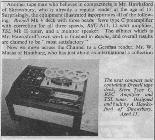
PHOTO 1: The 1963 article in HiFi News featuring 15-year- old Malcolm’s
integrated tape machine.
Using the (then new) emitter-coupled logic from Motorola, I was able to get up to 100MHz clocks, and that was in 1968 mind you. This logic family had to be interconnected using transmission- line techniques with proper termination to prevent reflections! This choice of subject proved rather fortuitous, as it gave me a strong grounding in delta- modulation and its close relation sigma- delta modulation, technology that was later to have a massive impact on audio systems in the 1980s and 90s.
JD: Do you see circuit design as an art?
MH: Yes, I think it is to some extend an art, or a bridge between science and art, in the sense that you develop a “pictorial” solution without knowing exactly how you got there. It sort of develops itself. I have been doing circuit design most of my life and it has become a “sixth sense”; I’m thinking in circuit blocks, sort of. In those early days you would try Out different topologies, thinking it through, and trying to picture the currents and voltages in your mind while trying to get to the optimal solution.
JD: Is there a personal style in circuit design? Is there a “Hawksford” style in circuit design?
MH: To a certain extent I think there is. Designers usually solve a circuit problem slightly different from each other, perhaps based on how they learned to solve certain problems earlier and probably also depending on their personality. If you are a digital designer, you might choose to plug some design spec into a program that puts it in an FPGA for you. Likewise, as an IC designer you may have a library of standard cells or modules that you can use to lay out your chip.
In each of these cases the designer seems a step or two removed from the detailed design, making it more anonymous, unlike an analog discrete circuit designer. That said, I think that also sometimes circuits are designed differently for other reasons than you might think. I firmly believe that if you design an amplifier, and you take care of both the critical factors and secondary effects, such designs will tend to “sound” very similar. . . hopefully implying the performance is accurate.
Now, of course, the topology isn’t all of it. People often become preoccupied with topology, but there are many more issues required to make a circuit into a great piece of equipment. There’s the power supply, the grounding layout, EMI issues, the quality of the components, the wire used—they all contribute to the final result. So, when you get the topology right—that is, get it to con verge in terms of stability and linearity and such—then the secondary factors become important.
Let me give you an example. Most designers are aware that you must avoid sharing supply return paths between power and signal returns. The power return current could cause a “dirty” voltage across the return path that couples into the signal circuit. Even if you use a series supply regulator, you can still have this problem with a rock-stable and clean supply voltage, because the harm is done through the return current.
Now, if you use a shunt regulator, the “dirty” current can be localized and kept from signal returns, and that offers a major advantage. If it still isn’t enough, you can use what is called an “active ground” or “dustbin” where the supply return current is not returned to the ground common at all but disappears into another, separate supply system (Fig. 1A-C).
JD: What is your view on the desirability and usefulness of blind testing to rate the performance of audio equipment?
MH: Well, I think you must use some kind of objective form of subjective testing method to isolate differences between components. Many people do not realize that they have a sort of internal perceptual model that determines how they perceive the auditive input. That internal perceptual model not only takes into account the sound feed from your ears into your brain, but also how you feel, your expectations, how bright is the environment, how relaxed you are, and many other factors. So if your internal perceptual model changes due to those other interference factors changing, your perception of sound can change.
I recall occasions where initially I perceived a certain difference between cables, and then I repeated it the next day and my perception was often quite different. I think this was due, at least in part, to my changed internal perceptual model. So some kind of objective test is required, but that said, I’m not a strong advocate of ABX-style double-blind testing (DBT).
The limitation in sensing a change in sound can put us in an unnatural situation, and I’m not sure we then function so reliably or sensitively. Possibly a better approach is a blind method that allows a relaxed and holistic type of listening session, Of course, with DBT it’s easy to get a null result, so it may be a good method if that is your agenda.
My preference is to undertake listening tests in a completely darkened room. The fact that the equipment you listen to isn’t hidden and could be identified with just a bit more light makes it much more natural and less stressful than being aware that the equipment is purposefully hidden from you. Also, being able to focus your senses purely on sound and not be distracted by uncorrelated visual input to the brain heightens your auditory perception. It is very easy to do and increases your sensitivity and acuity, especially in spatial terms.
In my experience it is not the same as closing your eyes. It seems that when you close your eyes when listening, you are sort of fooling yourself it’s artificial in a way and it still diverts some mental processing power away from your listening. You should try the dark room sometimes, although it’s good to keep a small torch at your side!
JD: Another method correlating measurements with perception that gets some attention lately is trying to extract the difference between the “ideal” signal and the actual signal. In the past year I attended several AES presentations on systems to extract those differences and make them audible, such as the differences between unprocessed music and the MP3 version. Bill Waslo of Liberty Instruments, the makers of the Praxis measurement suite, even has a free version online (AudioDiffmaker).
MH: It is a very powerful technique which I explored formally in 2005, and we have employed the extraction of error signals over many years at Essex (see, for example, “Unification” articles on my website). The idea is that you have a system with both a target function (the design response) and the actual function with imperfections, so you can then rep resent the actual system in terms of the target function and an “error function.” There’s a lot to it, but as a simple example consider the frequency response of a high-quality CD player. You can assume that the target response here is a flat response to around 20kHz; if that is not the case, then, of course, you need to correct for the nonlinear target response in the extraction of the error.
If, for example, there are response irregularities below; say, -40dB, it would give around 0.01dB frequency response ripple. You barely see that in the frequency response, as it’s actually less than the graph line thickness! However, if you assume a flat target response, extract the error and then plot it on the same graph, which tells you much more.
FIG. 2 shows the minute ripples in the response resulting from an imperfect DAC reconstitution filter. This tells you how far below the main signal you have some kind of “grunge” in the system, where ideally it should be below the noise floor. I like this type of presentation because it can inform you of the actual low-level error resulting from small system imperfections (both linear and nonlinear) that may cause audible degradation. This frequency response example is relatively simple, but in the paper I give some examples of using MLS or even music signals to extract the low- level errors from ADCs and DACs.
JD: If you can extract the error, can you then not compensate for it? Sort of “pre-distorting” the signal with the inverse of the error function? Possibly digitally?
MH: Well, compensating analog systems with numbers becomes complicated pretty fast. Most of these errors are dynamic or may arise from some interference of some kind, and although you can measure them accurately, you cannot predict them to any accuracy. The errors vary a lot with time and temperature and what have you.
It’s been tried with loudspeakers, where you can develop a Volterra-based model to describe cone motion, for instance, and use inverse processing to linearize it. But it is extremely difficult to keep the compensation model synchronized to the instantaneous cone position and movement. If you’re just a little bit off, the results may be worse than without correction. It’s much easier and cheaper to design a better driver!
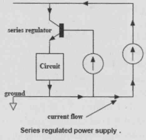
FIG. 1A: Series regulator return current flow.
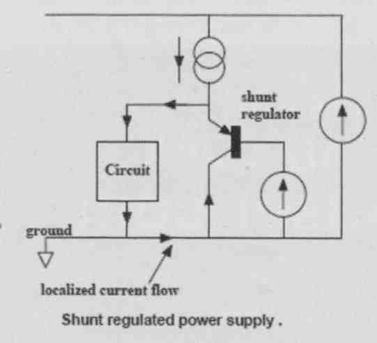
FIG. 1B: Shunt regulator localizes return current.
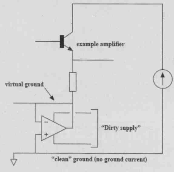
FIG. 1C: “Active ground” dumps re turn currents in another supply.
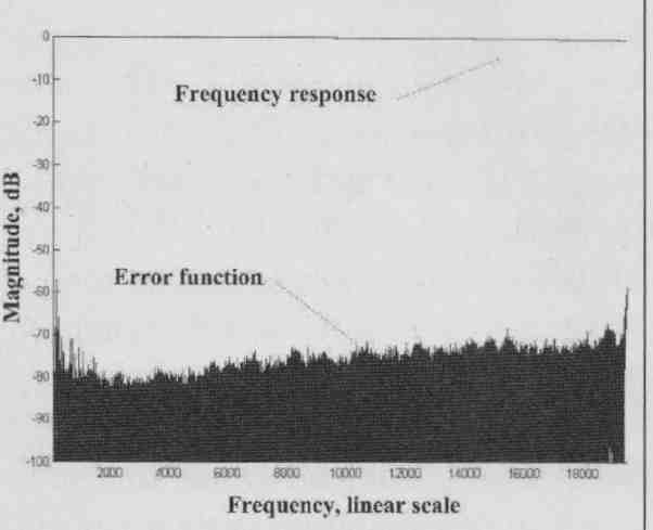
FIG. 2: Example error graph for CD frequency response.
There are some other techniques. There’s a guy called David Bird, who used to work for the BBC and was using a current drive technique. One of my ex-Ph.D. research students, Paul Mills (who is now responsible for loudspeaker development at Tannoy), and I have also done some work on that subject. With current drive, the principal error is, in fact, the deviation of the Bl -product of the driver.
You can therefore measure the BI deviation as a function of cone displacement, and if you then monitor the cone position, you can apply inverse Bl correction such that the force on the cone is proportional to the input current. We actually developed a transconductance power amplifier to current drive a loudspeaker, with several error correction techniques included in the design. We solved the low-frequency damping problem in two different ways. One was to use an equalizer; you measure the hi-Q resonance and then preprocess the signal to obtain the required linear response.
The other approach was to wind a thin wire secondary coil onto the voice- coil former of the drive unit, just voltage sensing, and to process that signal and feed it back into the transconductance amplifier. There was some unwanted transformer coupling from the main voice coil into the sensing coil which we had to compensate for with a filter. But since the main coil was current driven, it didn’t matter if it heated up, and since there was no current flowing through the sensing coil, it also did not matter if it heated up. It worked very well; I remember that even using current drive with a tweeter also significantly lowered distortion.
JD: It wouldn’t help with things like cone breakup.
MH: No, it wouldn’t. And it adds an extra layer of complexity and things that can go wrong. It is also only suitable for active loudspeaker systems.
JD: One issue that turns up in your work again and again has to do with jitter in some form.
MH: Well, yes, because it turned into an issue after we got the CD from Philips and Sony, and after the first euphoric reports, many people realized that what should have sounded perfect didn’t. A major cause was jitter, which hadn’t re ally been considered in those early years, probably because jitter is an “analog aspect” of a digital system. It can also manifest itself in different ways; it can disguise itself like noise (random and relatively benign) or as a periodic disturbance related to power supply ripple or clock signals, which is more objectionable, or it can be correlated with the audio signal, which also can sound quite bad.
So just saying “jitter” is not enough; its effect depends very much on how it manifests itself. In fact, I produced a paper at one time in which I designed a jitter simulator that allowed one to compute specific amounts and type of jitter, noise or periodic or correlated to the signal, and add that to the clean signal so you could listen to its effect (see sidebar Hawksford on the Sound of Jitter).
You can debate its significance, but at least you can point to a measureable and audible defect, whereas a traditional jitter picture with sidebands and what have you doesn’t give you a “feel” for what it sounds like.
I did a study with research student Chris Dunn (not the Chris Dunn who has published substantial work on jitter) which showed that the jitter introduced by the AES/EBU (or S/PDIF) inter face protocol even depends on the bit pattern—in other words, on the music signal itself.
For instance, when you listen to the error signal of the phase-lock loop (PLL) on the digital receiver, you can actually hear the music signal that was transmitted through that digital link! It is distorted, of course, but this was clearly an example of music-correlated jitter.
Now there are known engineering solutions to eliminate that jitter later on, but it doesn’t always happen in equipment, so there is the possibility when you transmit digital audio through a band limited link (and it is always band limited), you can get correlated jitter just from that process. We also showed that if you code the L and R signals separately, invert one of them, and then send both over that interface, almost all of that signal-related jitter would disappear. But it wasn’t picked up on; such is the law of standards!
JD: How would you design the “ideal” DAC?
MH: The DAC chips themselves nowadays are very good indeed. Where you see the differentiation in quality is in stages like the I/V converter, a seemingly innocent subject. The sharp switching edges from the DAC output can only be perfectly reproduced with an I/V op amp that has infinite bandwidth and no limit on slew-rate. Any practical circuit will have nonlinearity and slew rate limits such that a transient input signal can slightly modulate the open-loop (OL) transfer of the op amp.
Modulating the OL transfer function means you modulate the circuit’s closed-loop (CL) phase shift. What is interesting is that it looks remarkably similar to correlated jitter; they share a family resemblance (Fig. 3). It also is similar to what people have been talking about as dynamic-phase modulation in amplifiers. Whenever an amplifier stage needs to respond very quickly, it tends to run closer to open loop and therefore is more susceptible to open loop non linearity. So the I/V stage is clearly a critical stage, and although the underlying processes are different, the resulting signal defects may manifest themselves as correlated jitter, especially as the timing errors occur close to the sampling instants where signal rate-of-change is maximum.
Anyway, I really think we should not talk about phase modulation here, as that is more appropriate for sine wave signals and linear systems. We should talk about temporal modulation instead. There are many ways you can solve these issues once you understand them, possibly to design your I/V converter to be very wide band, or using a very linear open-loop circuit, or maybe some low- pass filtering between DAC and I/V stage. What you end up with is a discrete current-steering circuit that runs partially open loop and integrates the I/V conversion and low-pass filtering into one circuit, rather than bolting an I/V stage to a subsequent second-order filter as is normally done. Consequently, you minimize the active circuitry involved (Fig. 4).
If you think about it, theoretically we are trying to make circuitry work flawlessly up to infinitely high frequency, which in principle cannot be reached. So at one time I thought maybe we need a totally different way to solve the problem of critical timing issues in DACs.
One possible solution I came up with was to modulate the reference voltage of an R-2R ladder DAC with a synchronized raised-cosine waveform. Rather than the DAC output staircase signal jumping “infinitely” fast to a new level at every clock pulse, it effectively made the new level the same as the previous and then ramped it up, so to speak, to the new level using a raised-cosine shape with the same period as the clock (Fig. 5A, B). Consequently, adjacent samples were linked by raised-cosine interpolation rather than a rectangular step function. This also helps a little with signal-recovery filtering. So, the rate-of- change of the currents coming from the DAC was dramatically reduced. I built a prototype to proof the principle and it dramatically reduced the timing and transient errors in the I/V stage.
In many ways I view I/V conversion after a DAC as the digital-system equivalent of a MC phono preamplifier.
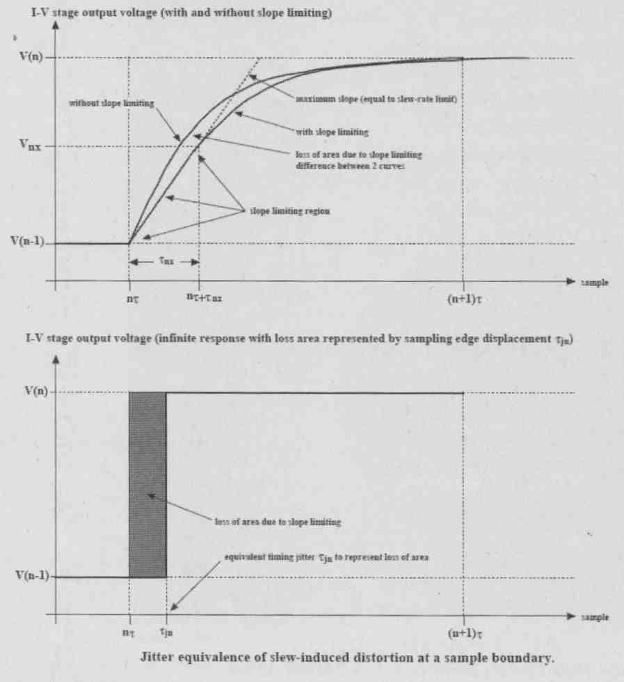
FIG. 3: Slew-rate limiting in I/V converters has jitter equivalence.
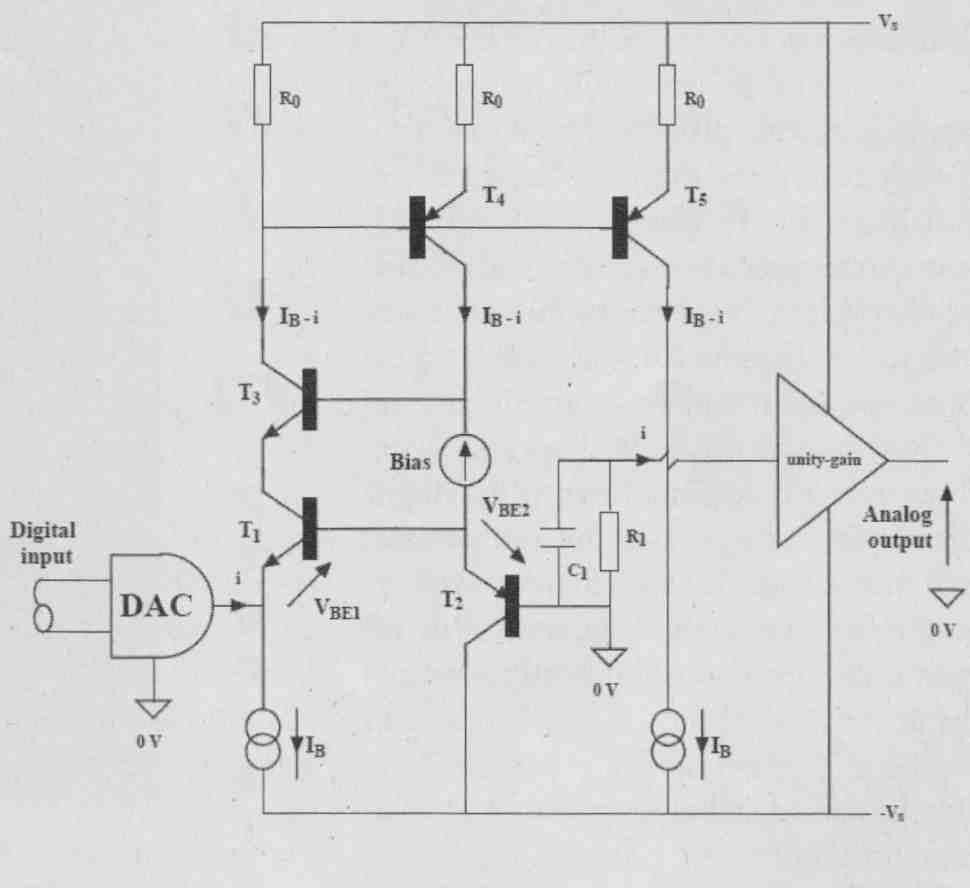
FIG. 4: An open-loop I/V converter with integrated filter and input-stage
error correction.
Although the application is totally different, I find that if you have learned to design a good MC preamp, that actually helps you to design a good I/V stage!
Another important issue is to locate the clocking source for the DAC very close to the DAC itself and slave every thing, including the transport, to that clock. The clock should be free running, very pure and not controlled by a PLL; very often a PLL will only move the jitter to another frequency band and the frequency of oscillation is bound to wobble. There’s nothing wrong with a free-running clock as long as you make sure that your data samples arrive on time, and you can do that with an appropriate buffer memory and data re quest protocol.
The CD player is a horrible RF environment, and you need to get the clock and DAC away from that source; just place a portable radio close to a CD player and do your own EMI testing! Even local supply bypassing of the DAC can couple noise into the supplies for the clock and increase jitter! So now you can list a few issues necessary to get it “right” in a digital playback system: the I/V; all the massive problems from EMI, supply, grounding, and so forth; and putting a clean clock right where you need it. I would speculate that if you gave a circuit topology to three different engineers to lay out a PCB and then build it, you would end up with three different results purely due to the differences in layout and component parts selection.
Now, how do you get a clean, stable DAC clock in your system? Suppose you have a transport and a DAC inter connected and you try to stabilize the DAC clock at the end of the digital interconnect; in principle you will succeed long-term, but in the short term that clock will wobble about and produce jitter. And even if you have your super DAC with clean clock and PLL with low filter cutoff, you still are faced with an input signal that is not necessarily clean. It can induce ground-rail interference and your supply may become contaminated, so that incoming jitter may then bypass all your hard work and still end up affecting the output of the DAC. Memory buffers can, of course, help in the smoothing process, but beware of power supply and ground-rail noise.
JD: Benchmark Media Systems claims that their DAC1 products succeed to almost get rid of jitter completely be cause they put a very clean clock next to the DAC with an option to slave the transport clock to it. Their USB interface apparently works the same in that it actually “requests” samples from the media player or PC, at a rate dictated by the clean DAC clock.
MH: Yes, network audio turns a lot of these issues upside down. It actually works the other way around. You put the DAC clock in charge, and it can be very clean and free running—no PLL—very low phase-noise. It is the way it’s done in the Linn Klimax DS; the clock effectively “demands” audio samples from the network or NAS drive at its own pace to keep the buffer memory filled. I found the Klimax one of the cleanest and most articulate digital replay systems I’ve ever heard. For me, this is the way to go.
Now, I think that a good high-resolution 24/96 or 24/192 audio file, de livered through a top-notch network DAC, can sound absolutely stunning, and I have some wonderful Chesky recordings at 192/24. But even a 16/44.1 CD recording, when played through a network DAC implemented correctly, can also sound pretty spectacular. Maybe not quite as good as the hi-res stuff, but very, very good nevertheless, and you would be hard-pressed to hear the difference. Of course, the CD recording quality has to be first rate, but that’s a very different story!
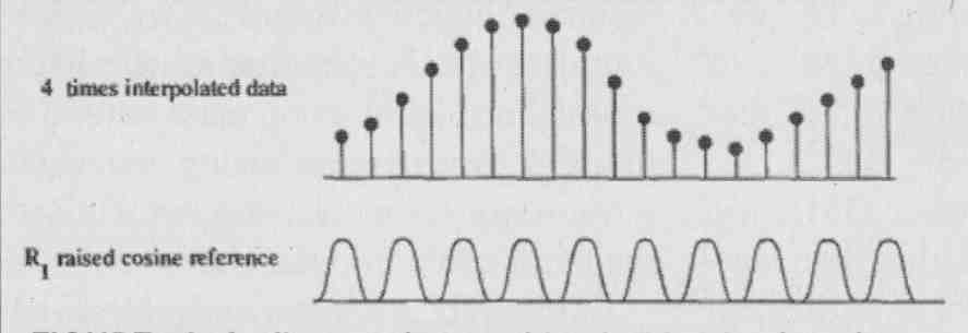
FIG. 5A: Audio samples combined with raised-cosine DAC reference combine
to …
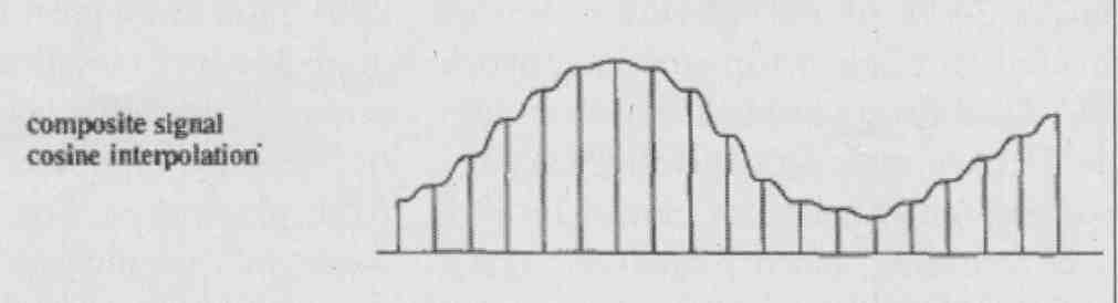
FIG. 5B: ...dramatically reduce harmonics in analog output current reducing
I/V slew rate requirements.
JD: There are several companies out there trying to make this happen. Mark Waldrep’s iTrax.com allows you to download music on a pay-per- download basis, where the price depends on the quality. You pay perhaps $2 for a 24/96 download, giving you actually the recording master, down to perhaps $0.69 for the MP3 version of the same music.
MH: Yes that’s an extremely good way to do it, and if you look at the Linn website you’ll see that they offer similar services. Linn also gives you the option to buy their hi-res content pre-loaded onto a NAS drive, which for some people is more convenient than the hassle of downloading and setting up playlists on the PC. Chesky Records is also a very excellent source of music, and they actually have some 24/192 material. The B&W model that you sub scribe to and obtain regular downloads is also interesting.
I think if you make the price right and especially if you provide high-quality recordings, people won’t cheat, generally. And these specialty music providers also are extremely careful about the recording quality of the music they list, so that is one more uncertainty removed from buying a CD, where you may like the music but maybe the recording quality isn’t so good. So to me it looks that networked audio delivery is slowly coming of age, yes.
JD: Can we spend a few words on loud speakers and their part of the audio performance? In your keynote speech to the Japan AES regional conference in 2001 you saw a great future to Distributed-Mode Loudspeakers (DML) to diminish the influence of room acoustics on music reproduction.
MH: Yes, indeed. You see, a DML has some great advantages. Rather than having a pistonic action like a traditional cone or panel speaker, a DML consists of a myriad of vibrating areas on a panel where in effect the impulse response of each of these small areas has low correlation with its neighbor. That is the significant thing which makes the polar response spatially diffuse. Now many people feel uneasy with that because it looks as though this will lead to a dif fuse field, and it does!
But, it does not lead to a significant breakdown of spatial sense or of instrument placing, because although the field becomes diffuse, the directivity characteristic does not. The major advantage is that the room acoustic reflections add with a significant degree of incoherence; they average out, so to speak, they are diffused. It helps to make an analogy between coherent light (from a laser) and incoherent light (from conventional lighting); in the latter the lack of interference results in much more even illumination without interference patterns.
To be honest, the sound stage itself does suffer a little bit, but the advantages can outweigh the disadvantages. You have no defined sweet spot, but you have no “bad” spot either when you move around the room. Furthermore, you could construct a DML as a flat panel, make it look like a painting, for instance, which makes 5.1 or 7.1 surround so much friendlier in the living room! You could even make them an integral part of your flat-panel video screen or, in principle, weave them into the fabric of the room architecture.
But as far as I know only NXT has taken up the technology for use in specific circumstances, and successfully, I might add. Now, for regular stereo use, DMLs may not quite give you the sharp holographic image traditional loud speakers can achieve, but in practice that will not often happen anyway. People seldom place their loudspeakers in the correct position in the room to realize the full potential for imaging.
Now that we are discussing the diffuse characteristics of DML loudspeakers, it reminds me of something similar I have done with crossover filters where the cross over transfer functions have a kind of random component added to them in the crossover region. The issue is: If you add the responses in a crossover on-axis, they add up and you should get a flat combined response. But if you add them off- axis, you normally would get a dip at the crossover frequency due to interference from non-coincident drivers. But with noise-like frequency responses, then for the off axis sum, the interference is dispersed and the dip spreads out over some frequency band around the cross over frequency and becomes less pronounced. You diffuse the problem, so to speak. It's similar to what DMLs do: I call them stochastic crossovers (Fig. 6A, B).
PHOTO 2: The Professor in his element: explaining feedback/feedforward concepts.
JD: You would favor active speaker systems?
MH: Yes. I believe that active loud speakers have a number of advantages due to using separate amplifiers for each frequency range. Intermodulation, either directly or through the power sup ply, is much easier to avoid, as different amplifiers handle different regions of the audio band. Amplifier peak power requirements are also relaxed, in turn making it a bit easier to build high- quality amplifiers. And, assuming close proximity between amplifier and its associated driver, then those pesky loud speaker cables are largely removed from the equation (smiling).
In the 80s I consulted on what I believe was the first digitally corrected active speaker, developed by Canon. In fact, Canon funded a research project at Essex where we (that is, Richard Bews, now proprietor of LFD Audio, and me) produced a system that was ultimately demonstrated at their research facility in Tokyo. [ I have listened to that system in a large room in a General’s castle in Belgium in 1984 or thereabouts; it left a vivid memory!]. There are two key aspects to digital loudspeaker processing. First, you can use it as a digital crossover filter, which will allow you to very easily correct any loudspeaker response errors as part of the crossover code. This is much simpler and less costly than using high-quality analog crossovers.
But once you have the capability the urge is often to use it for room correction as well. I’m not a fan of that, simply because (ideal) room correction can typically be done for only one specific listener location, the ubiquitous “sweet spot.” At any other location, the response, including the phase response, goes down the drain. The problem is very much wavelength dependent, so accurate correction tends to be limited to low frequency with less precise frequency shaping being applied at higher frequency. So, I’d use digital loudspeaker processing only for crossovers and loudspeaker correction. You should deal with room influences (other than low- frequency modal compensation) through other methods, where intelligent loudspeaker placement is one powerful way to improve your stereo reproduction.
Now, there’s another aspect to digital loudspeaker equalization. Loudspeakers are a bit like musical instruments really; they have their own coloration and character where often you chose what appeals to you. Now if you equalize that loudspeaker, you may compromise the attribute that you liked, so, although being more accurate you may have the impression something is missing or wrong. You should therefore consider digital loud speaker correction an integral part of the design, just as is a passive crossover.
You shouldn’t try to play with the correction or have switchable multiple corrections, just as you wouldn’t want switchable multiple passive crossovers (apart from maybe some slight level correction in the low- or high-frequency range).
JD: That’s the philosophy of AudioData in Germany. They sell one of these digital speaker/ room correction systems. They will come to your home and set the system up to your liking with the corrections and all. They do not encourage you to play around with it. They put your particular correction files on the Internet, so when some thing goes wrong in your system you can download and re-install them. But in a practical sense it is a one-time thing—to your room, your speakers, and your taste, if you will.
MH: Yes, that’s sensible. People should listen to the music, not to their loudspeakers or correction processing! There’s one more thing I’d like to mention about placement. In the past, I have worked closely with Joachim Gerhard (founder of loudspeaker company Audio Physic in Germany), who came up with one of the best placement schemes I know. You need to avoid reflections coming from the same direction as the direct sound, because this distorts your spatial perception (it messes with the head-related transfer functions we use in sound localization). Joachim drew an ellipse that just touched the inside of the room boundary. You then place the loudspeakers at the foci of this ellipse and place yourself at the middle of a long wall boundary (Fig. 7).
So, not only are the reflections now remote from the direct sound direction, they are also separated more in time, where both these effects have a major impact on localization and perception of the recording venue acoustics. In the context of a high quality two-channel audio system (using Audio Physic loudspeakers), it achieved one of the finest stereo soundstages I have ever heard. The sound seems to hang in there between the widely spaced loudspeakers; you can hear all detailed venue acoustics, very convincing, especially when the room is darkened! Also, having the loudspeakers widely spaced increases the difference signal between our ears, which helps to produce a more 3-D like image. Very interesting.
FIG. 6 A/B: Stochastic crossover has randomized filter characteristics
that diffuses the off-axis crossover dip.
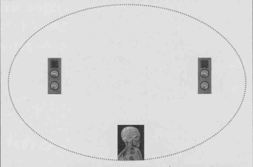
FIG. 7: Idealized speaker placing (Joachim Gerhard, founder of Audio Physic).
JD: Siegfried Linkwitz makes the point that you should place the speakers such that there is a minimum of 5ms temporal separation between direct and reflected sound, so that your brain can separate out the recording venue acoustics from the room acoustics.
MH: Yes, I very much agree with that. With most stereo placements, you add room reflections to the sound which “dilute” the spatial properties. So you may think that you have a larger image, but that is because it is blurred! The ellipse-based placement I just mentioned separates the direct and reflected sound both in direction and timing, and so helps your brain to keep the original spatial properties intact.
JD: And then there’s the issue of the speaker cables. I remember this paper you wrote in Marrakech I believe.
MH: I wrote a lot of papers in Marrakech! I like to get away now and then to a quiet place, away from daily distractions. I would get up at 5:00 am and then work for three or four hours. Those hours can be very productive, what you would call "quality time." But you probably refer to my article on cable effects and skin depth That one attracted a lot of criticism, and although there was a degree of speculation in it, I stand behind the major conclusions to this day. If I write something like that I always try to indicate what is fact, as we electronic engineers understand it, and what is more of a gut feeling, In that article I addressed the topic of skin effect in the context of audio; however, it seems what I said was widely misunderstood and misquoted. Say you have a coaxial cable, consisting of lossless conductors (i.e., zero resistivity). All AC-current would then flow only on the two opposing inner surfaces as electro magnetic forces would push the charge carriers away from each other; the current would not penetrate the conductor and skin depth would tend to zero.
Here all the electromagnetic energy would flow only in the dielectric space between the two conductors, propagating in an axial direction along the cable close to the speed of light with the conductors acting as guiding rails. Here the electric field is radial, while the magnetic field is circumferential with power flow in a direction mutually at right angles to these two fields that is along the cable axis. Now because all practical conductors are lossy, you inevitably get potential differences along each conductor, and this means that at the cable surface there must be a component of the electric field in an axial direction; however, the surface magnetic field is still circumferential.
When you consider these two fields, the direction which is mutually at right angles is now directed in a radial direction into the interior of each conductor.
As a consequence, there is a propagating electromagnetic wave (loss field) within the conductor itself. Think of it as energy spilling out into the guiding rails which are now partially lossy and therefore must dissipate some energy.
When you solve Maxwell's equation for propagation in a good conductor, you obtain a decaying wave be cause some energy is converted into heat. Also, the velocity is very slow and frequency dependent. It is this slowly propagating wave that determines the internal current distribution in the conductor and is the basis of skin depth; it also explains why skin depth increases with decreasing frequency. The "loss field" is at maximum at the surface and decays exponentially into the conductor.
So your current is no longer con fined to the conductor surface but penetrates into the conductor; it depends on frequency and decays exponentially. Therefore, when you consider the series impedance of a cable, you find it is made of two principal parts. There is the inductive reactance due to the magnetic field within the dielectric between the conductors, and this, as you would expect, rises as 6dB/octave. However, the magnetic flux trapped inside the conductors has both a resistive and an inductive component. If the skin depth is such that the current has not fully penetrated all the way to the center of the conductor, then this component of impedance approximates to 3dB/octave.
What happens in practice depends on the actual cable geometry and there- fore which aspect of the impedance is dominant. I could go on, but I suggest you download “Unification” from my website for more information. So to conclude, at lower frequency the penetration is deeper while as frequency rises, the internal conductor impedance increases as the current becomes more confined to the surface layer, just as it would be if the conductor was lossless to begin with.
I also put some numbers to it and it turns out that when your conductor diameter is less than about 0.8mm, there are almost no skin effects even up to 20kHz.
Now, going back to loudspeaker cables, ideally you would want them to have just a very low value of resistance over the audio frequency band with no reactance. Due to the phenomena described above, that may not always be true, but there lies the art of loud speaker cable design!
However, in understanding the problem with loudspeaker cables that can impact their perceived subjective performance, there is another important factor. Even if cables are completely linear, they still feed loudspeaker systems that offer a nonlinear load due to drive unit impedances changing dynamically with cone displacement, suspension nonlinearity, and possibly saturation effects in crossover components. As a result, the current entering the loudspeaker is a nonlinear function of the applied voltage; this, in turn, means that any voltage drop across the (even perfectly linear) cable also has a nonlinear component which must be added to the loudspeaker input voltage. It is interesting to audition these error signals in real-world systems where distortion can be clearly audible. So in this sense cables do impact the final sound where this process is probably responsible for perceived differences in character or coloration.
= = = =
HAWKSFORD ON THE SOUND OF JITTER
There is a, lot of talk about the effect of jitter on reproduced music. To help people to get a feel for it, I prepared some test files with well-defined amounts of jitter. Basically, what I did was to calculate the variation in digital sample values when a specific jitter signal would be present, and alter the samples accordingly. The tracks are audioXpress .com/files/hawksford_jittertracks.zip">here and can be listened to or downloaded for your own use. Those of you adventurous enough to go through the details are referred to the reference below.
Track 0 is the original music, and the following tracks are the resulting amplitude-normalized “distortion” or error signals resulting from the types of jitter as listed:
Track 1: TPDF (triangular probability distribution function) noise-based jitter
Track 2: 2 equal-amplitude sinewaves (44100 - 50) Hz and (44100 + 50) Hz based jitter
Track 3: 3 sinewaves 50Hz, 100Hz, and 150hz, amplitude ratio 1:0.5:0.25 based jitter
Track 4: sinewave 0.2Hz based jitter
Track 5: sinewave 10Hz based jitter
Track 6: 3 equal-amplitude sinewaves 1Hz, 501-li, and 44100/4Hz based jitter
Track 7: All of the above 6 jitter sources combined.
NOTE In a real-world situation these error signals require amplitude scaling to match the system jitter level; they have been normalized here to allow them to be auditioned.
Enjoy!
Reference: Jitter Simulation in high-resolution digital audio, Presented at the l2l AES Convention, October 5-8, 2006, San Francisco, Calif.
= = = =
REFERENCES:
1. “System Measurement and Identification Using Pseudorandom Filtered Noise and Music Sequences,” JAES, Vol.53, No.4,2005 April.
2. “Transconductance Power Amplifier Systems for Current-Driven Loudspeakers,” JAES, Vol. 37, No. 10, 1989 October.
3. C. Dunn and M. 0. J. Hawksford, “Is the AES/EBUI’SPDIF Digital Audio Interface Flawed?,” presented at the 93rd Convention of the Audio Engineering Society, JAES (Abstracts), vol. 40, p. 1040 (1992 Dec.), preprint 3360.
4. Discrete integrated I/V
5. Ultra high-resolution spatial audio technology for HDTV on DVD, keynote speech at AES 10 regional convention, Tokyo, Japan, June 13-15,2001.
6. “Digital Signal Processing Tools for Loud speaker Evaluation and Discrete-Time Crossover Design,” JAES, vol.45 no.1-2, 1997Jan./Feb.
7. Electrical Signal Propagation & Cable Theory, Malcolm Omar Hawksford, October 1995, available online at stereophile.com
8. Bits is Bits? This work was funded by the UK's Science and Engineering Research Council, and was originally presented as a paper, "Is the AES/EBU S/PDIF digital audio interface flawed?" (Preprint 3360), at the 93rd Audio Engineering Society Convention, October 1992, in San Francisco.
Note: All papers referenced here and many more are available at Professor Hawksford’s website,
No, on to ...
Audio According to Hawksford, Pt. 2
JD: Let's move to amplifier electronics, because one thing that comes across clearly from your publications is that you enjoy electronic circuit design.
MH: Is it that clear? But it is true. My first amplifiers were tube-based, of course, and I still have a certain fondness for them. Most were simple, first-order circuits, with some pleasant coloration usually added by self-induced microphonics and vibrations. Different manufacturers using different tubes even with similar circuits show up different issues, but they err benignly, so to speak. It is very seldom that a tube amplifier's sound can't be enjoyed despite its technical limitations; the errors tend to be quite musical.
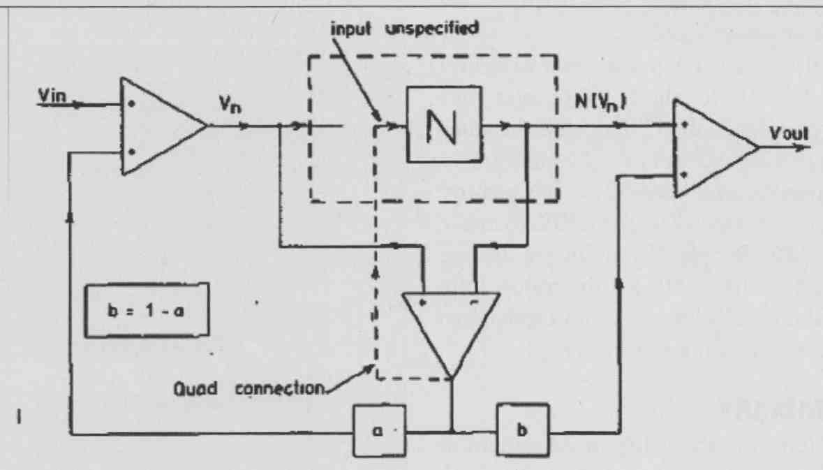
FIG. 8: Generalized ff-fb error correction structure.
JD: What triggered your interest in error correction (EC)?
MH: Peter Walker's Current Dumping concept did that. I thought it an extremely clever and elegant solution (still do), and a "thinking out of the box" amplifier de sign that was en vogue at the time. There are various ways of looking at Current Dumping, but I explained it as a combi nation of feedback and feedforward techniques. The clever bit, as I saw it, was that it allowed you to design a structure that didn't require infinite gain to obtain theoretically zero distortion over a fairly broad bandwidth. In a feedback amplifier, as you move up in frequency, the feedback decreases leading to increasing distortion.
In this (then) new concept, the feed-forward path compensates for the loss of feedback with frequency, and in theory you can keep up the "zero distortion" over the audio band. Of course, it depends on what stage of the amplifier produces distortion. It started me thinking about some way to generalize the concept of combining feedforward (if) and feedback (fb)-which, of course, is at the core of Current Dumping-and explore other trade-offs in ff and fb. As the most objectionable distortion in a power amplifier is generated in the output stage, would it be possible to locally correct that output stage so that the remaining distortion signals that are fed back from the output to the input stage would be much cleaner (i.e., devoid of output stage distortion) thus also contributing to lower input-stage distortion? As N (the uncorrected output stage gain) approximates to 1, the error tends to zero and this makes the difference (correction) amplifier much more linear as it only amplifies small signals, and this holds even when the output voltage swing is large.
The conceptual view (Fig. a) made it clear that, in theory, combining ff and th can completely eliminate the forward loop nonlinearity, without the need for infinite loop gain, simply by choosing suitable combinations of transfer functions a and b in Fig. 8 providing (a + b) = 1. Practical ff or lb networks will most probably need to have some active components and will thus be at least first-order low-pass circuits. But, if the "a" network has a first order 1/(1 + sT) characteristic, you could make "b" a conjugate sT/(1 + sT), and the elimination of distortion independent of frequency still holds.
Now, for the feedforward component “b,” there is the practical problem of combining the forward and feedforward signal in the output (power) stage, so that is less attractive. Therefore, one solution would be to use only the “a” lb path, as it is much easier to combine low-level signals at the amplifier input. Because you now can no longer compensate for the first-order rolloff, the full curative properties of the system break down at higher frequencies so zero distortion is out of reach.
Yet, employing this type of error correction locally in, for instance, output stages still has significant advantages. Such fast- acting local correction does a good job to linearize the output stage by one or two orders of magnitude and, as a bonus, give very low output impedance before global feedback is applied. I also showed that you can implement a correction circuit virtually without needing more components than those used for biasing, so it’s essentially free.
The local loop does not impact stability much, so you can have your cake and eat it, too. You end up with a more linear power amplifier for the same parts investment and that’s always worthwhile. Bob Cordell had a very elegant implementation of this concept which I like very much..
JD: At one point there was a great discussion on diyaudio.com between Bob Cordell, yours truly, and other very smart circuit designers. The question was whether error correction is really a different circuit concept or whether it is another way of using negative feedback (nfb). That it was, to paraphrase evolutionary biologists, a matter of exploring the “space of all possible nfb implementations.”
MH: Well, I guess that conceptually it is indeed a different way to apply nfb, but with some interesting different issues which also lead to more insight into this type of circuit. For instance, in Fig. 8, assuming that b = 0, then Vout/Vin = G = NI (aN - (a - 1)).The target for Vout/Vin = 1, so now you can calculate the error function representing the overall input- to-output transfer function error, that is the deviation from “1,” thus c is defined as c=1-G.
Substitution gives you C = (a - 1)(N - 1)/(aN - (a - 1)). Now you immediately see that the error function has two zeros, i.e., (N - 1) and the balance condition represented by (a - 1). This succinctly explains the operation and power of EC, especially with near unity-gain output stages as you get two multiplicative terms in the error function which should both be close to zero. Half of the art of understanding and developing circuits lays in finding the right viewpoint!
JD: I know of at least one commercial implementation of what appears to be your EC concept, based directly on Bob Cordell’s circuits, by Halcro. Presumably based on a patent by Candy, which came later in time than your publication.
MH: Yes, I am aware of that. At the time I sent Halcro my papers and wrote t them asking for some clarification, but never received a reply. So it goes. Anyway, life’s too short to worry about such things. It’s not my problem. Bob Stuart of Meridian Audio also used the circuit in his amplifier range for a period of time, which was most gratifying as he is a very gifted audio circuit and system designer.
There’s analogy to error correction in the digital domain, and that is noise shaping. I wrote a paper with John Vanderkooy comparing digital noise shaping with nested differential feedback in analog circuits and concluding that they can be seen as different views of similar issues! If you look at a first-order noise shaping con figuration (Fig. 9), you see that, similar to EC, you take the difference between the forward block (the quantizer) input and output, which is the noise it generates, and feed it back to the input, properly shaped like H = e^(-sT). Now, if you look at the noise shaping transfer function (1 - H), it looks very similar to the error reduction function of EC you showed before. So as you go lower in frequency, where the loop gain gets higher, the noise also gets lower.
Now this is a simple first-order case, but as you go to higher order noise shapers, your in-band noise gets lower at the expense of forcing more and more noise above the audio band. Now, if you put in a coefficient in (1 - H) of less than 1, then the reduction curve bottoms out at lower frequencies, so it is analogous to the bottoming out of your EC curve due to a less than 1 error-feedback coefficient. So, you could say that quantization noise shaping in sampled data systems is analogous to distortion-shaping in feedback or error correction in continuous signal systems. You often see that when the distortion is driven down by feedback or EC, it works for the first few harmonics at the expense of increasing higher harmonic components. Again, just like what we observe with noise shaping in digital systems!
You should look into the literature about Super-Bit Mapping (SBM). Michael Gerzon and Peter Craven in the UK worked on that as did Stanley Lipshitz and John Vanderkooy and also SONY. I well remember a rather heated argument between Michael and a Sony engineer during an AES convention some years ago! The idea with SBM is to apply noise shaping to a digital signal in the context of CD. Normally, with uniformly quantized and dithered 16-bit/44.1kHz LPCM, the noise floor is essentially flat from DC to 22.05 kHz.
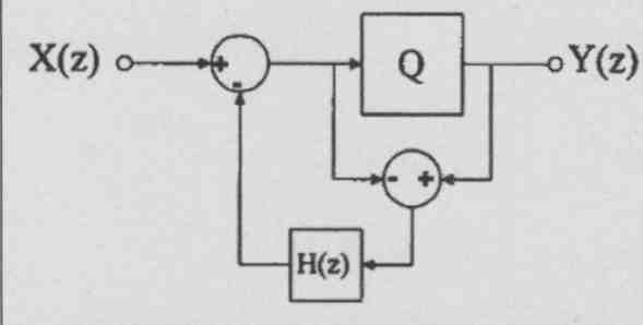 FIG. 9: Generalized noise-shaping structure.
Now, they asked, suppose we start with a 20 or 24-bit source, and we re-quantize and noise-shape the signal, can we somehow retain some of those additional bits of resolution below those 16 bits? Of course, the noise that you reduce in one part of the spectrum needs to go somewhere, and what SBM does is to decrease the noise in the mid band so you get perhaps 18-bit resolution in the frequency region where the ear is most sensitive.
The noise-shaping transfer function is designed to follow closely the Fletcher-Munson curves; consequently, the noise may rise by perhaps as much as 40dB at the very high frequencies, but because your ears are very insensitive in that area you cannot hear it. It is also important to realize that in a properly designed SBM system the noise is of constant level, and there should be no intermodulation with the signal. Also, the signal-transfer function is constant. So, provided that your DAC has at least 18-bit accuracy, you can perceive a subjective resolution of around 18 bit. And at its core, again, is a concept that you would recognize as an error-correction amplifier!
Your use of that AD844 current conveyor in your error-correction amplifier does remind me of a similar topology that I developed with two of my research students, Paul Mills and Richard Bews. This design, which led to the LFD moving-coil preamp, was published in HiFi News in May 1988. Richard subsequently developed this conceptual LFD pre-pre that used floating power supply circuitry by optimizing component selection and over all construction to achieve a very high level of performance. The reasoning behind the circuit is as follows: In a simple, single-ended emitter follower (Fig. 11 A) the transconductance of the stage Gm = + RE) where re is the intrinsic base resistance.
Since re = 25/I_E, you see that because re changes with signal current, this introduces distortion. You can improve on this (Fig. 11B), and now Gm = 1/ (r_e1 + r_e2 + R_E), where, for example, when r_e1 increases, r_e2 falls. There is not perfect cancellation because the transistors of the long-tail pair are effectively connected in series in the AC-equivalent circuit, but it is much more linear than the previous case. You can further improve on that with Fig. 11C, where complementary transistors are now effectively in parallel for AC, so the changes in the respective res due to signal current are almost perfectly complementary such that the transconductance of the combined transistors is almost independent of signal current; that is, the circuit is linear.
If you plot the nonlinearity (as an error function) versus the value of RE and signal current (Fig. 12), you see that there is a point, with very low RE, where the Fig. 11 C stage is almost perfectly linear. So this is a valuable property, but as you can see there are some challenges in biasing it, especially with those very low-value emitter resistors. However, you can rework the circuit to retain the linearity yet make biasing somewhat easier.
Another most important aspect of the topology is the use of truly floating power supplies because even if the supply voltage were to vary or to exhibit noise, there is no signal path linking to the RIAA impedance, as related currents can only circulate in closed loops. Consequently, power-supply imperfections are dramatically reduced, which is very critical in MC applications where small signals can be sub microvolt in level.
Under large signal conditions, you have transistor slope resistances and slope capacitances which are being modulated by the signal, and that’s potentially bad news. Some people call it phase modulation, going back to something Otala brought up many years ago.
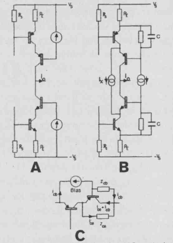
FIG. 10: Enhanced cascode concept.
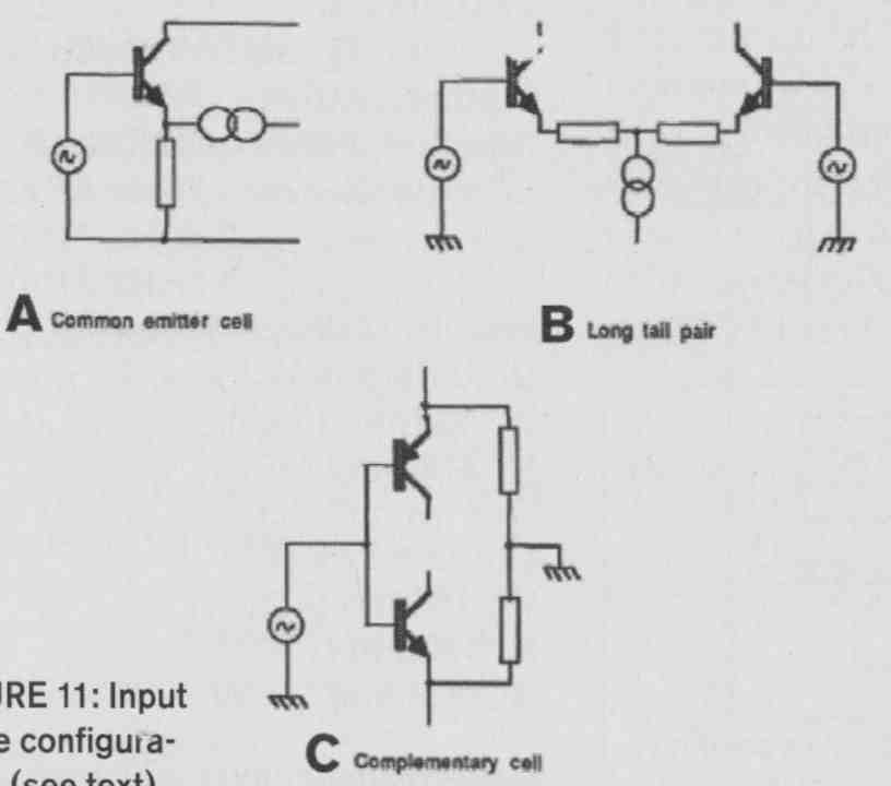
FIG. 11: Input stage configurations (see text).
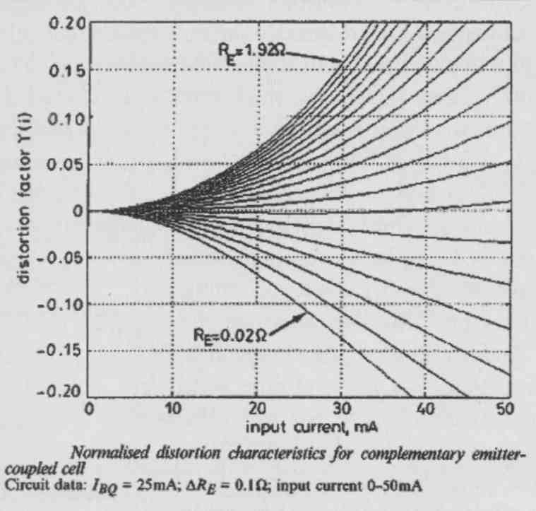
FIG. 12: Input stage linearity versus RE.
It’s more like a gain-bandwidth modulation, and I prefer to think of it as a time-domain modulation. For instance, in a feedback amplifier, this would slightly modulate the open-loop gain-bandwidth product and you can then calculate what it does to the closed-loop phase shift. It’s like a signal-de pendent phase shift, which manifests itself as jitter. It is analogous to a signal-dependent jitter, and it basically happens in all analog amplifiers. So, you have jitter in digital systems, you have jitter in I/V converters due to finite slew rate leading to slight modulation of the loop gain-bandwidth product, and you have these signal-dependent jitter- like phenomena in analog amplifiers in general, albeit that the modulation is time continuous rather than being instigated at discrete instants.
You know, if you start to design a system, you need to have some sort of philosophy that drives you. For me, it is often the minimization of these timing errors, and I think that large-signal nonlinearity is less of a big deal than sometimes is believed. Most of the time you listen to low- level signals anyway, where linearity is very good. So then, you ask, what distinguishes one system from another, right in these low-level regions?
Now, I don’t have any magic number, but let’s assume that 100pS is the magic number for digital jitter, and suppose that you find similar numbers for what I call “dynamic timing errors” in analog amplifiers, the picture sort of comes together. It just might be that simple, open-loop circuits, while having higher large-signal level distortion, potentially have less of these timing nonlinearities, which could explain their very good sound. I would need to get the sums together, but it just might be possible that this is one of the reasons why people prefer those simple, low-feedback amplifiers. Especially in transistor circuits, where the transistor parameters themselves are modulated by changing voltage and current.
So having simple circuits that minimize these changes and are designed to minimize power supply influences clearly helps. Of course, feedback can help in many ways and there is no fundamental reason that a feedback amplifier cannot exhibit exemplary results, providing care is taken to minimize modulation of the amplifier loop transfer function.
Another example: When Paul Mills was still at Essex, he was working on an amplifier design using a cascode stage (Fig. 10A) that had reasonably low distortion. Then I told him, “Look, Paul, I will make one modification to your circuit that lowers the nonlinearity by an order of magnitude!” What I did was re-locate the biasing for the cascode to its emitter rather than to the supply (Fig. 10B).
It doesn’t look like much, but it is a very significant change, and I can explain it with Fig. 10C. Why is the Z of a cascode not infinitely high and its distortion zero? It has to do with transistor slope parameters and their modulation with signal level.
You can see that an error current that is the difference between the ideal output (collector) current and the actual one is a result of the non-infinite impedances between emitter-collector and base-collector of the cascode transistor, where in Fig. 10C these two impedances are modeled by Zce and Zcb The modulation of transistor slope parameters with signal level I mentioned can be described as modulation of Zce and Zcb. So, if you could find a way to prevent these error currents from ending up in the output (collector) current, then their bad influence would be eliminated.
Now, what is the effect of re-locating the bias to the emitter instead of the supply? For example, the cb error current now no longer comes from the supply but from the emitter of the top transistor. ‘It is subtracted from its emitter current, which is basically the same as the cascode collector output current. So when is added to the cascode output current, it is no longer an error but makes up for the current that was subtracted in the first place! For a similar reasoning can be made. So the error currents now circulate locally in the stage and don’t contribute to the output. It doesn’t work perfectly, because there are some minor errors due to base currents, but it is, nevertheless, a huge improvement. The output impedance goes up typically by a factor of 10, and the distortion goes down by a factor of 10!
Note that it does not matter whether these error currents have a nonlinear relationship to the signal, as they do not contribute to the output current. This technique therefore works well in large signal amplifiers. I just picture this process in my mind, and I “see” what’s going on, and then the solution pops up.
JD: You need to make the mental leap to model this modulation as an error current, and then find a way to shunt that error current away.
MH: Yes, indeed. There are some issues involving stability, as there is some form of regeneration in the circuit, but that’s the gist of it. Now, I often wonder whether I would have seen that if I had plugged it into a simulator and run a distortion analysis. I like to think that I might not have made that connection. I also believe that you should lay out the PC board, build your designs, and think about the topology at the same time. The days of a light box and black tape were great and very intuitive, very human. You move the layout around, changing this and that and in some way that connects back to the circuit again and you may then end up improving the circuit. It’s an iterative process that can give you just that extra bit of quality or performance that you don’t get when doing a sim and then saying, well, that’s it.
Anyway, this particular enhancement then appeared in my enhanced cascode paper’°. Also, Richard Bews and I used this concept in the LFD preamp (Fig. 13), which, as previously mentioned, employed a true floating power supply system. And even if those batteries were to intro duce some supply voltage nonlinearity, this doesn’t show up in the output signal. There are no grounding problems because of the floating supplies. The floating-bias input pair is coupled to a cascode stage.
It’s clear that any changes in that bias voltage do not have any influence on the output signal. So this will have high output impedance which drives current into the passive RIAA network to convert that current to voltage.
Now, if you look at which components determine the sound quality, it’s only the input transistor emitter resistances and the components of the RIAA network. The cascodes don’t do anything; the power sup plies don’t do anything, so it’s an extremely linear circuit overall. And because it is only those few components, Richard was able to optimize component selection, ending up with a truly world-class preamp. Richard really is extraordinarily good at tuning and laying out circuits, and the battery-powered pre amp worked extremely well. Also, this is why LFD Audio now enjoys almost Cult status with its amplifier products.
JD: That Fig. 13 circuit looks deceptively simple, but it is a very intricate circuit, isn’t it?
MH: Yes, it is very simple, yet has a lot of interesting points: low noise, low distortion, almost no supply interaction, virtually no ground-rail current, very insensitive to transistor parameters, accurate RIAA correction, yet only a few active devices.
Often manufacturers have a good basic topology, but then they need to work in the power supply and grounding as well as the electrolytics and the other components in the signal path, and it all tends to blur the final sound. If you have many components in the signal chain, individual optimizations have relatively small impacts. But with this simple circuit, the components that determine the quality are few, and thus optimization has a relative large effect as well.
The absence of power supply interaction, however, is key to its performance. I find that at least as important as the topology itself, not only in preamps, but also in DACs and power amplifiers, for that matter. A lot of the differences between equipment in terms of clarity and cleanliness have to do with internal EMI issues and the power supply interactions and ground contamination.
JD: Well, we’ve already covered a lot of ground, but perhaps I can ask you about your views of switch-mode amplifiers.
MH: As you know, I’ve done a lot of work on Sigma-Delta (SD) modulation over the years. There is one proposal using an SD modulator driving an output stage with a pulse-density modulated signal. Now, the switching frequency would generally be higher than in the case of a PWM stage.
As you mentioned before, there is a basic problem with these types of circuits with EMI, and a higher switching frequency doesn’t help. Do you remember our discussion with raised-cosine modulation in a DAC? Well, in this particular idea I used something similar. Instead of supplying the switching output stage with a stiff supply, you use a resonant supply synchronized to the switching frequency of the amplifier. The supply voltage would, in effect, be a raised cosine, so that at each switching instant the supply voltage would be zero, and would then smoothly rise toward the full value (Fig. 1 4A).
The result is that EMI problems are greatly reduced because the switching effectively occurs at zero voltage, and the harmonics are both lower in level as well as much lower in bandwidth. The output voltage of the amplifier is now no longer rectangular but somewhat sine- shaped (Fig. 14B). Switching efficiency of the output stage is improved as well, and not only are those switches still either fully on or fully off but because switching occurs with zero voltage across the device, power dissipation in the finite switching transition region is reduced. The average output level of this scheme is somewhat lower than a regular PWM amplifier, but that can be compensated for as described in the paper.
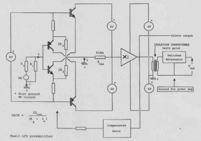
FIG. 13: LFD preamp simplified diagram.
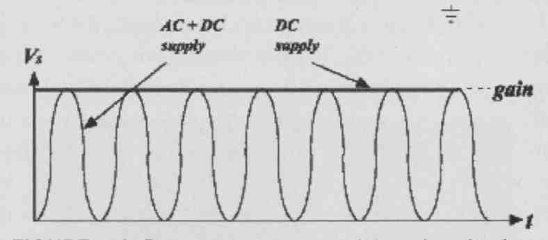
FIG. 14A: Resonant power supply synchronized to sample rate outputs raised-cosine
voltage.
FIG. 14B: Raised-cosine supply for switching amp dramatically reduces
output signal bandwidth.
JD: Do you think that these switched- mode amplifiers can reach the quality levels of a good analog amplifier?
MH: Well, I’ve heard some commercial systems with B&O IcePower modules, which seemed to work really well, so I would say it’s getting there, yes. It’s an interesting technology, and even if the samples I’ve listened to were not always very low distortion, they did have a certain cleanliness and transparency to them. I’m not absolutely sure, but it may be related to the absence of low-level analog problems like dynamic modulation of device characteristics in an analog amplifier.
So, I’m fairly optimistic, also because it brings the digital signal closer and closer to the loudspeaker, skipping analog pre amps and the like, Of course, you need to distinguish between “analog” switching amplifiers and “digital” switching amplifiers where the power amplifier is, in effect, the DAC. I have always been more interested in the latter class, especially the signal processing needed to achieve good linearity Just because an amplifier uses switching techniques does not necessarily make it a digital amplifier. This is an important distinction which is often misunderstood.
JD: Bruno Putzeys, a well-known de signer of switching amplifiers, maintains that switching amps are analog amps: they work with voltage, current, and time—all analog quantities.
MH: Indeed. So, there are still a lot of problems to overcome, but they have a philosophical “rightness” about it.
JD: Not the least because of the high efficiency!
MH: Of course. And even if you want ultimate quality, running your amp in class- A with a 500W idle dissipation doesn’t solve your quality issues either. There’s much more to amplifier quality than just the choice between class-A or class-AB/B topology An AB/B amplifier, properly implemented, with attention to all the often misunderstood issues of biasing, power distribution, grounding, and so forth, can sound so good that there is nothing to be gained by going to class-A. It’s better to go for a simple system, with as few stages as possible because an additional stage cannot fully undo any damage done by a previous stage.
Now, a great-looking box with lots of dials and lights certainly may play music well, but for ultimate quality, get the best DAC you can afford (preferably a net worked DAC linked to a NAS drive!), followed by a passive volume control and a great power amplifier and, of course, keep the cables short. Nothing can beat that, in my opinion.
JD: Professor Hawksford, thank you very much indeed for many hours of your time, for most interesting and illuminating discussions. In particular, I was intrigued by the correspondence between seemingly disparate phenomena, like noise shaping versus error correction and jitter versus analog phase modulation. I hope this will inspire readers to do their own experiments and come up with yet other interesting configurations.
REFERENCES
8. A MOSFET power amp with error correction, presented at the 72 AES Convention, Anaheim, 23-27 Oct. 1982, revised 25 Jul. and 27 Oct., 1985. Also on this web page.
9. Relationships between digital noise shaping and nested differentiating feedback loops, presented at the 93 AES Convention, San Francisco, 1-4 Oct., 1992, revised 9 Nov. 1999.
10. “Reduction in Transistor Slope Impedance- dependent Distortion in Large Signal amplifiers,” JAES, Vol. 36, no.4, April 1988.
11. “Dynamic model-based linearization of quantized pulse-width modulation for applications in DA-converters and digital power amplifier systems,” JAES, Vol. 40, no.4, pp. 235-252, April 1992.
12. “Linearization of multi-level, multi-width digital PWM with applications in DA conversion,” JAES, vol. 43, no. 10, pp. 787-798, October 1995.
Note: All papers referenced here and many more are available online.