|
|
Here’s a method to perform accurate noise measurements.
Conventional digital voltmeters (DVM) are incapable of measuring RMS noise beyond a few tens of kilohertz. Even expensive DVMs such as the Hewlett-Packard 3478A, 3456A, or Tektronix DM511 suffer from bandwidth limitations, some of which are “baked in” for RFI avoidance, and others attributable to the deficiencies of the RMS converter. Jim Williams of Linear Technology discussed the shortcomings in a paper, “Performance Verification of Low Noise Low Dropout Regulators.”
In addition to the shortcomings of random signal measurement, Dolby, Robinson, and Gundry in “CCIR/ ARM Practical Noise Measurement” found that unweighted and A-weighted noise measurements did not correspond well to the human perception of noise in recording. The authors suggest a circuit for a CCIR-ARM weighting filter and measurement regimen that addresses the problem. This paper was written at the dawn of cassette recording, and noise in the vicinity of 6kHz was thought to be under-measured by the systems employed at that time.
What’s a DIY audio enthusiast to do? In measuring noise, you could use a preamplifier such as Dennis Cohn’s low noise measurement amplifier employing the LSK389 dual JFET, or Geller’s “JCan” using the BF244A JFET, in conjunction with the RMS detector described here. I have used both the LTC1966 and LTC1968 from Linear Technology and the performance exceeded my expectations, surpassing all of the conventional digital voltmeters I have on hand, and approaches that of the two thermopile “true RN’IS” meters, a Fluke 8920A and Hewlett-Packard 3403C, which we employ for RF measurement. The CCIRIARM filter used in conjunction with the RMS detector will allow you to more knowledgeably measure audible noise in your system.
THE CCIR (ITU) ARM CURVE
Dolby’s paper includes a complete discussion of the benefits of the CCIR. Very briefly, un-weighted noise measurements are useful in the laboratory when bandwidth is specified, but of very little use in audio. A-weighting, adapted by the National Association of Broad casters, is based upon measurements of ear-sensitivity (Fletcher-Munson characteristics) and was widely used, but did not correlate well with the observed impression of noise experience. The DIN standard of the time, relying as it did on expensive (at the time) quasi-peak reading measurement, was dismissed owing to limited manufacturing sources and “unappealing” measurements. (In plain English, the DIN standard, if applied to manufactured products of the time, would have resulted in noise figures several decibels worse than advertised.)
The authors recommended the CCIR response curve, one which features a somewhat exaggerated response from 2 to 12kHz, together with an average-responding RMS milli-voltmeter. The “zero loss, zero gain” frequency of the CCIR filter was selected by Dolby as 2kHz and is illustrated (with this adjustment) in comparison to the A-weighted curve in Fig. 1.
The effects of repetitive impulse noise are understated with an average responding meter, but the authors demonstrate that the differences are close to constant. Thus, the response is compensated by 6dB to take into effect the difference between measurement regimens. The zero-crossing point was shifted by Dolby from a nominal 1kHz to 2khz to avoid measurement problems associated with the particular shape of the curve.
A complete description of the noise measurement method is contained in “Measurement of Weighted Noise In Sound Program Circuits, ITU-T Recommendation J.16, which is available on the ITU website. The paper also contains tolerances at discrete frequencies from 31.5Hz to 31.5kHz. The circuit in Fig. 2 is used to specify the ITU recommendation J.16.
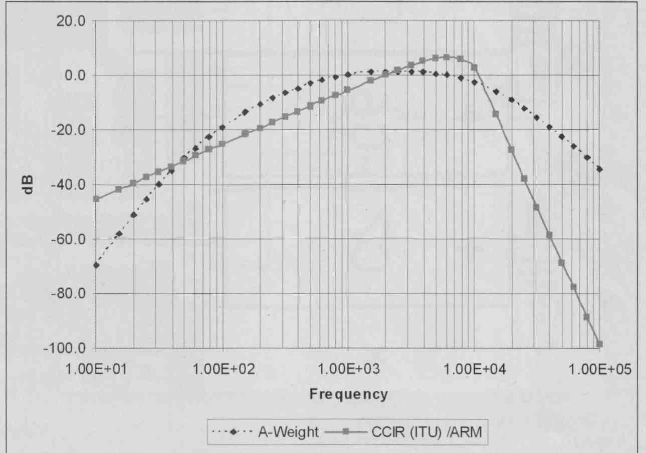
FIGURE 1: Weighted and CCIR filter response.
IMPLEMENTATION
In the Dolby paper the authors showed how to implement the time constants of the filter with a discrete component design consisting of a 7-pole low-pass filter and 1-pole high-pass filter. Simulating their design, I found that the filter was optimized for the 0.0dB shoulder points of the bandpass response.
Today, the filter may be fashioned with operational amplifiers. For the most part, I used the filter values of R&C described in the JAES preprint. Not surprisingly, the CCIR filter for my Boonton 1120 Distortion Analyzer used virtually the same configuration, and the schematic I utilized and show is only slightly different from the Dolby and Boonton designs. The Hewlett-Packard (now Agilent) 8903 Signal Analyzer also used a somewhat different arrangement. The HP 8903 CCIR-ARIVI filter is available on the web.
U1A is a first-order low-pass filter with an f3 of 10.6kHz. P1 may be adjusted for 12.2 or 17.8dB gain at a frequency of 6.3kHz. The shoulders of the response curve will then fit close to 0.0dB at 1.0 and 12.5kHz for the ITU Standard or 0.0dB at 2.0 and 10.9kHz for Dolby’s implementation. (In this example, I set the shoulders at 1.0 and 12.5kHz.)
The other opamps are 2nd-order Chebyshev low-pass filters with approximately 0.6dB ripple. Feed-forward (R13, R14) was used by Dolby to taper the response from 9.0 to 31.5kHz. The high-pass filter formed by C2, R1, and P2 shapes the response to a bandpass filter conforming to the ITU standard.
P2 may be adjusted (as described later in this article) to shift the high-pass response so that symmetry between the 1.0 and 12.5kHz shoulders is attained, The schematic is in Fig. 3.
The values of R13 and R14 differ from those of the JAES preprint. I found that 392 ohm and 95.3k-ohm yielded a falloff more consistent with the theoretical values of the LCR filter in the ITU standards. The value of R13 influences the slope of the low-pass filter and can be adjusted to suit your pr I have used values from 27k to "open." The choice of op amps is not that critical, provided that the gain bandwidth product is sufficient.
RESULTS
The filter performs quite well in comparison to the theoretical values. The performance is illustrated in Fig. 4.
The ITU J.16 specification states the tightest tolerance, 0.0dB error at 6.3kHz. The gain of each filter can be adjusted for exactly 12.2dB gain at this point. The gain at 1.0kHz should then be 0.0dB within a tolerance of ±0.5dB, and 0.00dB at 12.5kHz with a tolerance of ±1.2dB. The operational amplifier filter fits well within the specified tolerance bands as illustrated in Fig. 5. The tolerance bands specified by the ITU are shown for reference.
I have also provided results for the op amp filter without feed-forward (triangular marker). The error in this case is very low for almost the entire curve, but breaks the band at 20.0 kHz by about 0.5dB.
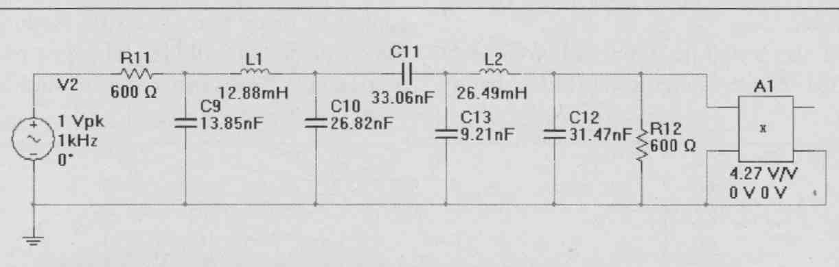
FIGURE 2: Circuit used to specify ITU recommendation J.16.
The discrete design schematic in the JAES preprint is a bit difficult to read, and the slight variance from that of the op amp design may be attributable to errors in reading the circuit diagram from an original that was not well copied. These are simulated results (Dolby Sim, circular marker), not a device that is actually bread-boarded, so reality and SPICE may not necessarily be on the same page. The authors allowed trimming resistors in several locations that would benefit the already good performance.
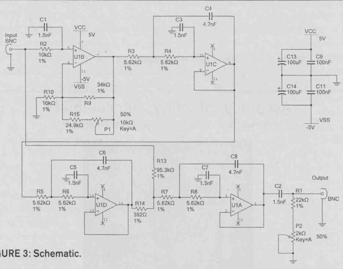
Fig. 3 Schematic
I also tested the filter with a GenRad 1381 Noise Generator (50kHz bandwidth) and an HP3577 Network Analyzer (Fig. 6).
SETUP AND USE
While the setup should be straightforward, you may prefer to use the “snip-able” machined IC socket pins for placement of R13 and R14. You can then experiment with values to render an optimal response.
Use of a voltmeter with a dB function is most helpful. In this case, apply a 1.000V 1.0kHz signal to the filter and set the dB “relative” to measure 0.0dB at this frequency. Next, measure the output at 6.3kHz, which should be approximately +12.2dB. If the 6.3kHz output is too low, adjust potentiometer P1 (gain adjust) to bring it to +12.2dB. Reduce the frequency to 1.0kHz and adjust potentiometer P2 to bring the reading at this frequency to 0.0dB.
By adjusting potentiometer P2 (symmetry), gain at 1.0kHz and 12.5kHz can be balanced. When you adjust P2, however, the 6.3kHz gain will also change, so you need to twiddle the little potentiometers until you have a happy menage à-trois among the 1.0kHz, 6.3kHz, and 12.5kHz settings of 0.0dB, +12.2dB, and 0.0dB. For relative measurements, the filter set up this way correlates very well with the ITU standard. (To match the Dolby CCIR-ARM setup, the 0.0dB crossing points are shifted to 2kHz and 10.9kHz by adjusting the gain of the amplifier.)
If your voltmeter does not have a decibel function, start by setting your function generator for a 1.000V output at 6.3kHz. The output at 1.0kHz and 12.5kHz should be 0.2455V at each shoulder frequency, a level that is -12.2dB from the value at 6.3kHz. You will need to adjust potentiometer P2 to arrive at the blissful settings just mentioned.
The feed-forward network of R13, R14 adjusts the slope of the low-pass filter. Without R13 (infinite resistance) the results were very accurate, except at one data point, 20.0kHz. You can try different resistance values to come up with a filter shape that Suits your purpose (the easiest being elimination of R13!).
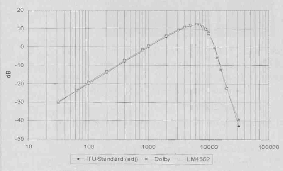
FIGURE 4: CCIR-ITU ARM filters.
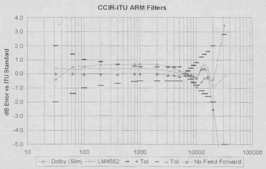
FIGURE 5: Discrete Dolby filter compared with operational amplifier.
TRULY MEASURING AN RMS VOLTAGE
One of the reasons for writing this article was my desire to use Linear Technology’s LTC1966 or LTC1968 “True RMS Detectors.” Even high-quality digital multimeters are woefully inadequate when attempting to accurately measure voltages above a few kilohertz or to measure complicated or random voltages. Above some 10s of kilohertz, the performance of many very high-quality voltmeters are compensated to eliminate the influence of radio frequency and electromagnetic interference. Figure 7 demonstrates the frequency limitations of popular meters, along with the superiority of “truly true” RMS meters such as the Fluke 8920A and Hewlett-Packard 3403C, or the RMS measurement function on the Tektronix TDS3012B oscilloscope.
The “log-antilog” RMS converter, usually an Analog Devices AD536 used in the HP3478A or Boonton 1120, doesn’t cut it when it comes to making noise measurements over a few tens of kilohertz. On the other hand, the Fluke 8920A and HP3403C meters, using thermopile true RMS detectors, excel but are very difficult, probably un-repairable if the thermopile is damaged. Jim Williams of Linear Technology points out their measurement superiority in his aforementioned application note, “Performance Verification of Low Noise, Low Dropout Regulators.”
Recently, Linear Technology introduced the LTC1966, LTC1967, and LTC1968 true RMS detectors. These replaced the now obsolete LT1088, a thermally responding true RMS detector that was discussed in AN-83. The LTC1966, 7, and 8 use a proprietary (and patented) delta-sigma modulation technique in which the converter’s output is equal to (V The output is averaged with a capacitor that forms a low—pass filter.
The description of the operation of the device is beyond the scope of this article, and I refer you to the product description on Linear’s website. The LTC1968’s modulator clocks 0.8pF at 2MHz, while the LTC1966 clocks 2.5pF at 100kHz. Linear indicates that the LTC 1966 has greater linearity than the LTC1968 but more limited band width. On the other hand, the LTC 1966 can use ±5V DC supplies, while unipolar operation of the LTC1968 is recommended.
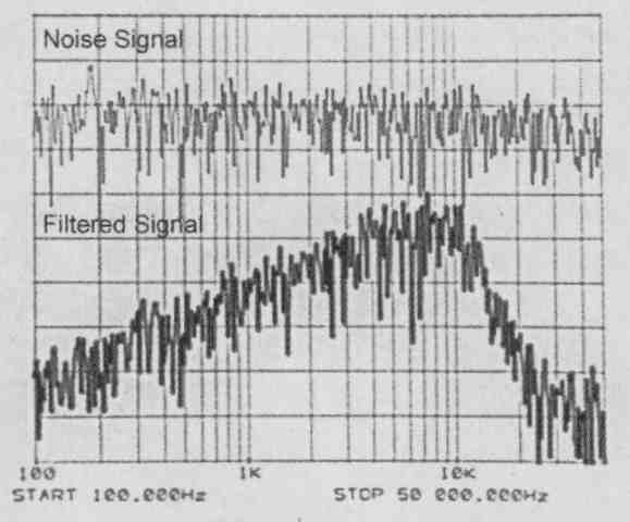
FIGURE 6: Testing the filter with a Gen rad 1381 noise generator (50kHz band
width) and an HP3577 network analyzer.
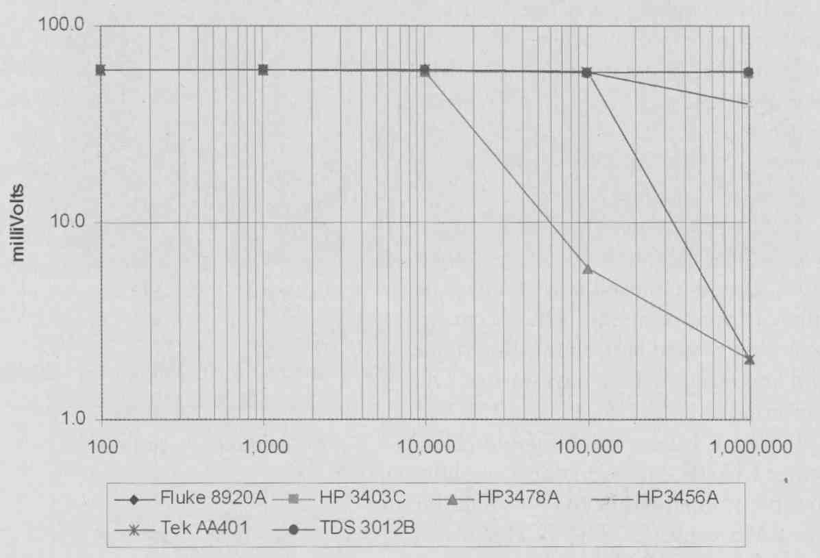
FIGURE 7: “True RMS” meter performance.
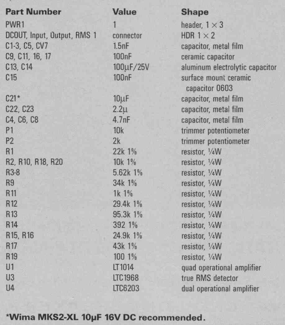
These devices require a bit of care and feeding for proper use. First, they are packaged as MSOPS, which makes a printed circuit board a necessity. (You can get around this by purchasing the development board sold by Linear). Second, I found that the best results were obtained when the device input was buffered with a simple non-inverting op amp. Third, a quality averaging capacitor such as a polycarbonate, polypropylene, or polyester type will improve accuracy. WIMA recently introduced its MKS2-XL series, which offers a 10uF 16V DC PET capacitor in a MKT07X9R5 profile, which I use as the averaging capacitor.
Last, ripple is present on the output due to the switching action of the modulator. This is removed with a low-pass filter. I found that the “DC-Accurate” post filter worked best, eliminating ripple and rendering a very easy-to-use DC converter.
I used a Linear Technologies low-power LT6203 dual operational amplifier to serve as input buffer and post filter for the RMS converter. The PCB shows a through-hole DIP pinout. I simply used the LTC6203 on an SOIC-DIP adapter. The schematic for the buffered and filtered RMS converter using the LTC1968 with a single supply (and LT6203 with dual supply) is shown in Fig. 8.
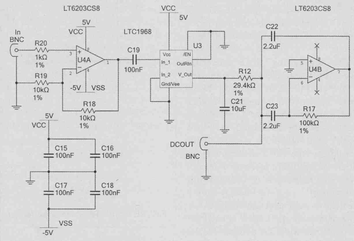
FIGURE 8: Schematic for buffered and filtered RMS converter using the LTC1
968 with a single supply (and LT6203 with dual supply).
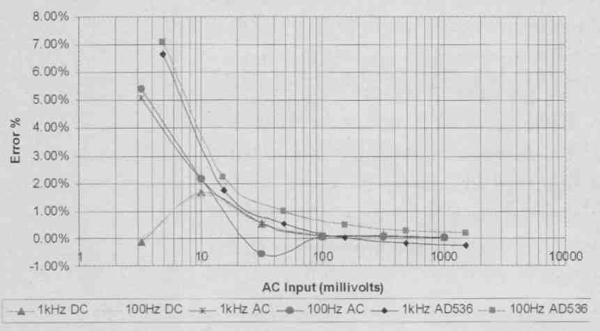
FIGURE 9: LTC1 966 and AD536 performance.
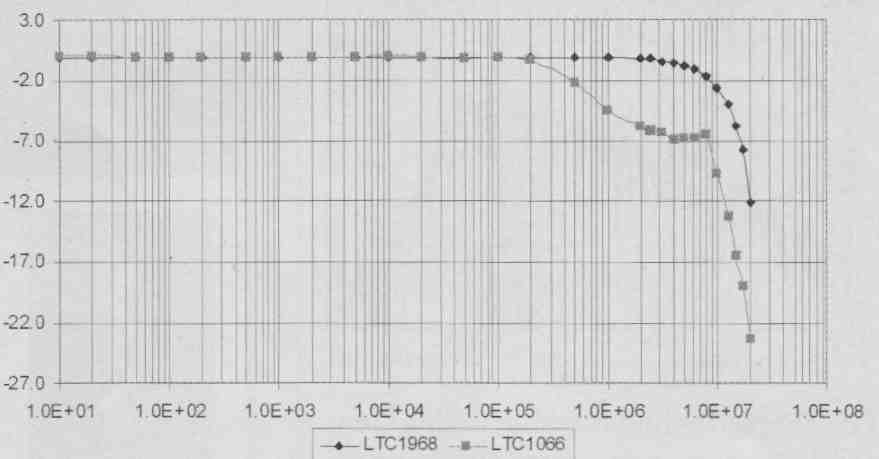
FIGURE 10: LTC 1966 and 1968 bandwidth (measured with DC Accurate filter).
RESULTS:
In an input range of 100mV to 1000mV, the errors for the LTC1966 average approximately 0.07%. Figure 9 illustrates the errors for DC- and AC-coupled situations of both the LTC1966 and the AD536.
The data in the LT product folders is formatted in terms of absolute error, not relative error. Figure 9 certainly con firms the excellent performance of the RMS converter for voltages greater than 100mV. The comparison between devices is on an apples-to-apples basis, using the post filter and averaging capacitor recommended by ADI, but without offset trim.
--- PARTS LIST - --
BANDWIDTH
The LTC1968, used on the development board with the DC accurate filter option switched in provides accurate measurement to 1.0MHz, and is down 3dB at 12MHz (Fig. 10). The LTC1966 on the filter PCB is a bit more constricted in its bandwidth, but according to Linear, more linear. The peculiarities in the response curve of the LTC1966 may be owing to my own “inartful” design. Either filter chip would be good in the measurement of audio noise, but the LTC1968 would be preferable in a digital voltmeter, or in the gain control circuitry of an oscillator.
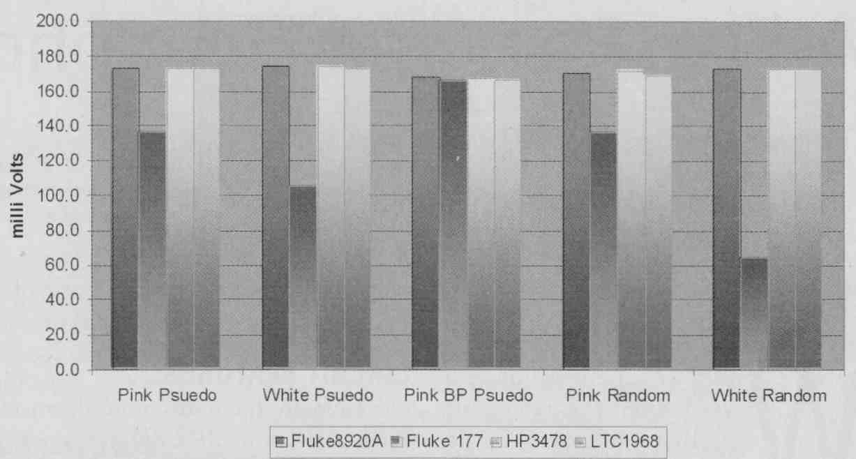
FIGURE 11: True RMS detector comparison.
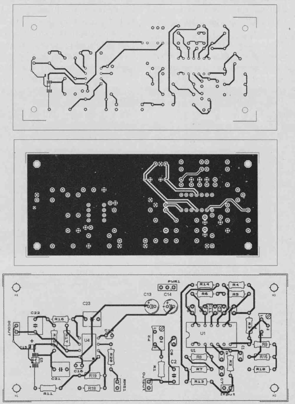
FIGURE 12: Printed circuit boards: top, bottom, and silk (stuffing guide).
A TOUGHER TEST
The Audio Precision System 2022 analyzer provides several flavors of random and pseudo-random noise. Figure 11 compares the LTC1968 with the Fluke 8920A, HP3478A, and my handheld Fluke 177.
The conclusion is pretty evident. If you choose to measure noise in your system, be aware of the limitations of the RMS detector in your measurement instrument. The LTC1966 and LTC1968 chips from Linear Technology offer great performance at a comparatively low price. Furthermore, the use of the CCIR-ARM filter will help you to accurately measure the noise you may or may not hear!
Test equipment used in this article includes: Audio Precision System 2022 analyzer, Boonton 1120 Analyzer, Hewlett-Packard 3336B Synthesized Level Generator, Hewlett-Packard 3577A Network Analyzer GenRad 1384 Noise Generator, Fluke 8920A True RMS Meter, and Tektronix TDS3012B Oscilloscope.
PRINTED CIRCUIT BOARD
Both circuits can be fashioned on one printed circuit board measuring 4.5 by 2.0”. The top, bottom and silk (stuffing guide) are illustrated in Fig. 12.
REFERENCES
1. Williams, Jim, “Performance Verification of Low Noise Low Dropout Regulators,” Linear Technology Corporation Application Note 83, March 2000.
2. Dolby, Roy; Robinson, David; Gundry Kenneth; “CCIR/ARM: A Practical Noise Measurement Method,” Audio Engineering Society Preprint 1353, May 1978.
3. Cohn, Dennis, “A Low-Noise Measurement Pre-amp,” audioXpress , April 2007.
4. Geller, Joe, “Build the JCAN to Measure Resistor Noise,” Nuts and Volts, July 2007, pp.
5. The URL for the standards wiki Standard: ITU-R_468. The URL for the ITU is www.itu.int.
6. Agilent put the HP8903 service manual on the web at www.agilent.com and inserting 8903 in the search engine.
= = = =