High Fidelity. To many people, both in and out of the radio profession, the great advantage of FM lies in its ability to reproduce the full range of audio frequencies. For sales appeal, the term "high fidelity" was popularized and everything desirable was associated with it. And yet, like everything else that has been oversimplified, unwarranted assumptions have been made.
High fidelity represents not one but a host of ideas, and what may appear to be high fidelity to one person may not be so to another. To a large extent, high fidelity involves the listener, and thus any complete consideration of the meaning of this phrase must not only include the technical details of the electrical system but the relationship of the listener himself to the system.
It is because of this latter aspect that we find any one precise definition of high fidelity impossible. Nonetheless, we may still investigate the contributing factors which add up to provide good reproduction of a broadcast.
Briefly, these factors include the electrical system (receiver and transmitter), the loudspeaker, the surrounding acoustics of the room where the re production occurs, and, finally, the aural capabilities of the listener.
In considering the listener, we find that the human ear has a frequency response characteristic that varies not only with each individual but also with age and even slightly with the length of time that the ear is subject to the music or speech of any one continuous listening. As an example of the average frequency characteristics of the ears, consider Fig. 10.1. Here we have the different intensities which each frequency must possess in order to sound the same to our ears as the 1000-cycle note. An example will perhaps make this clearer. Dealing with the bottom curve, we note that a 50-cycle note must be 50 db stronger than a 1000-cycle signal in order for both sounds to seem equally intense to us. Each curve represents the response at different sound levels. Thus, the bottom curve is for very soft sounds, almost at the threshold of audibility. The top curve represents situations where the sound is so loud or intense that hearing involves pain. The other curves are for intermediate degrees of intensity. In each curve, the 1000-cycle frequency is taken as the level of reference. From these curves, several important general conclusions may be drawn.
1. The best response occurs around 3000 to 4000 cycles.
2. The low frequency response is poorest at low intensity levels. Thus, when the volume is turned down low the low frequency notes suffer the most. Many manufacturers incorporate compensation for this in their tone controls.
3. The overall ear response is flatter as the volume increases. Note that the curves near the top of Fig. 10.1 tend to be fairly flat.
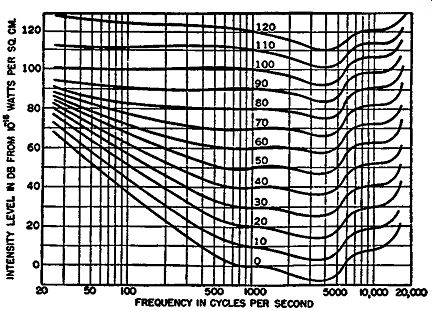
Fig. 10.1. Frequency and loudness characteristic curves of the ears,
as obtained by Fletcher-Munson.
Although not indicated in the diagram, individual hearing ability de creases with age. As one grows older, the ability to hear any of the audio frequencies deteriorates, with the higher frequencies subject to the greatest loss.
To consider only one of the foregoing conclusions, provision must be made in the radio receiver to compensate for the change in hearing response at different volume levels. As mentioned, most manufacturers incorporate low frequency compensation on volume controls at the lower level. Beyond this, however, very little has been done and the listener is obliged to resort to his tone control for further adjustments.
The dependence between volume and the frequency response is indicated more clearly in Fig. 10.2. Two curves are shown, one for the average listener and one for the more critical listener. The data for the average-listener curve were obtained by using people of all ages and both sexes. We see that, when the sounds are very loud, the frequency range for the average person extends from 20 to 15,000 cycles. As this volume is decreased, both ends of the curve drop and the frequency response becomes narrower. As before, the ear is most sensitive to frequencies between 3000 and 4000 cycles.
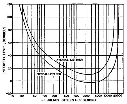
Fig. 10.2. A comparison between the hearing ability of average and critical
listeners.
In the discussion of these curves, no mention was made of noise, which is present to a certain degree in all homes. The surrounding, or (as it is more technically known) ambient, noise will be most noticeable when the volume is turned down low. It will tend, also, to mask the low and high frequencies because, as we have seen from the charts, these require greater intensity to produce the same aural sensation. It has been discovered that the average residential noise level is 43 db. In many homes, with children romping about, the noise is considerably higher and the ability of a person to hear is that much more impaired.
The Loudspeaker. As a converter of electrical currents into acoustic sounds, the speaker is as much an integral part of this system as the listener.
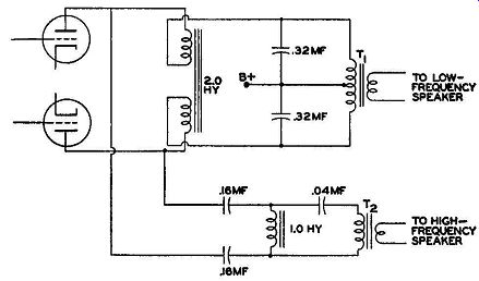
Fig. 10.3. A frequency-dividing network designed to feed two speakers.
In midget sets the small diameter cones are capable of a restricted range with best response at the frequencies between 4000 and 5000 cycles. Since it requires a large cone area to reproduce effectively the low frequencies, high fidelity reproduction from these small sets is impossible. In console receivers a popular solution to the problem of efficient reproduction is through the use of two speakers. A frequency-dividing network, shown in Fig. 10.3, separates the frequencies as they come from the output transformer and thus permits each speaker to respond only to frequencies within its designed range. Another approach is with a coaxial speaker, where one small cone is positioned at the center of a much larger cone (see Fig. 10.4). Again, frequency-dividing networks provide each speaker with its proper band of frequencies. The name "coaxial" is derived from the similarity of this arrangement to the coaxial cable where one conductor is located at the center of an outer hollow conductor.
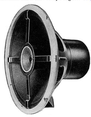
Fig. 10.4. A coaxial type of speaker. (Courtesy of ,Jensen.)
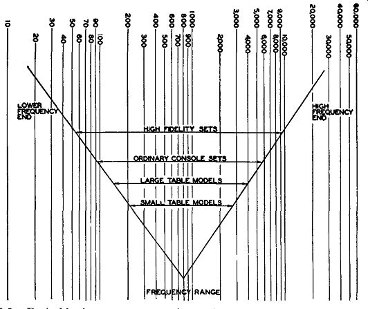
Fig. 10.5. Desirable frequency ranges for various types of receivers
in order to obtain the proper tonal balance.
Balance. It is common belief that everything less than the full frequency coverage of 30 to 15,000 cycles leaves us short of our goal of high fidelity.
Extensive tests have indicated, however, that of greater importance than trying to establish the maximum range is the balance achieved between the highs and the lows. By balance, we refer to the low and high frequency limits of our system. If we take a system and extend the high frequency response without providing a corresponding extension at the low frequencies, we find that the results do not tend to be as pleasing despite the fact that, from a true fidelity viewpoint, we are now in a position to receive more of the audible frequency range. The aural effect of extending the high frequency end, for example, without similar compensation at the low frequency end is to give the speaker response a shrill tone. Small radios possess speakers that accentuate the higher frequencies. This requires frequent use of the bass portion of the tone control to produce a compensating mellow effect.
The concept of balance has not been reduced to a definite mathematical formula, but it has been suggested that a good, empirical test is to have the product of the high and low frequency limits of the band fall approximately between 500,000 and 600,000. Thus, as an illustration, a band that starts at 90 cycles at the low frequency end should extend up to 6000 cycles at the high end in order to preserve the balance between the upper and lower limits. The chart in Fig. 10.5 shows how the limits vary from a small table model to a large console radio with a proper balance maintained in all in stances.
Bandwidth Limits. It has been assumed throughout the foregoing discussion that the receiver networks are fully capable of passing all the signal sidebands. Although this may readily be accomplished if the manufacturer takes the proper precautions in design, the simple fact remains that this is not so in many instances. The proper bandwidth response must be maintained in the R.F. and I.F. transformers, in the audio amplifiers, the output coupling transformer and, finally, in the loudspeaker itself. In the tuned coupling transformers of the R.F. and I.F. stages, the usual arrangements result in the familiar, rounded response. With this response, the lower audio frequencies which arc closest to the center of the carrier (hence closest to the center of the curve) receive the greatest amplification. The higher frequencies, situated farther away, receive correspondingly less amplification.
Hence, even if the signal is properly balanced at the set input, by the time it reaches the second detector the balance is distorted because of unequal amplification accorded the various frequencies. These are the present conditions in AM receivers. With an FM receiver, unequal response in the R.F. and I.F. circuits does not greatly affect the signal as long as its strength is sufficient at the limiter to cause saturation. However, in an FM receiver, the bandpass of each tuning circuit must be wide enough to permit reception of the full 200 khz, and the discriminator must be capable of converting FM to AM linearly. Careful design and construction are needed to balance all these factors-a fact that frequently varies in direct proportion to the price of the receiver. The latter statement is not meant to be an indictment of present practice but merely a recognition of some of the commercial considerations that often waylay high fidelity.
We have touched briefly on the subject of high fidelity to indicate some of the highly personal factors that combine to form this concept. It is be cause individual tastes differ that we find an extensive use of tone controls in most FM receivers. Some of the common methods of achieving this tone variation will be taken up in a later section.
Phase Inverters and Push-Pull Amplifiers. In order to be able to produce the full range of audio frequencies at full volume without undue overloading, push-pull output amplifiers are required. Advantages of push pull amplifiers arc (1) the cancellation within the stage of second harmonic distortion, (2) greater permissible drive at the input producing a stronger output with less odd-harmonic distortion, and (3) smaller output trans formers and less supply voltage filtering. The last advantage reduces hum and permits a greater dynamic range from the loudspeaker. At low volumes, hum can be very disturbing, and the current practice of accentuating the bass response of a receiver by special cabinet construction tends to accentuate hum further. In a balanced push-pull amplifier, a-c ripple from the power supply is eliminated in the plate transformer.
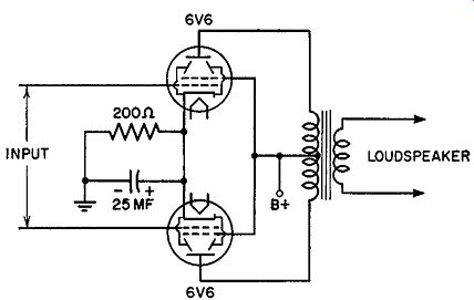
Fig. 10.6. A push-pull amplifier.
If we use a push-pull stage, such as the typical unit shown in Fig. 10.6, then the input voltages to each tube must be 180° out of phase with each other. The simplest, although not the cheapest, means of accomplishing this is by using input transformers. Ordinary transformers, however, have a poor frequency response, and compensated transformers are quite costly. The best solution is the use of a phase inverter whereby a portion of the signal is taken and inverted so that it becomes 180° out of phase with its input signal.
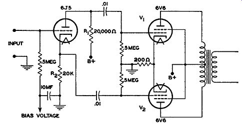
Fig. 10.7. Phase inversion supplied by a single triode.
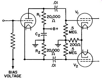
Fig. 10.8. Fig. 10.7 rearranged to emphasize the balance of voltage
across R1 and R2 .
This makes available two properly phased signals for the push-pull input.
Present phase inverters fall into several categories. The simplest arrangement is shown in Fig. 10.7, where a single triode (6J5, 6C5 etc.) sup plies both out-of-phase voltages. One push-pull amplifier receives its excitation from the plate of the phase inverter; the other push-pull tube receives its signal from the inverter cathode. That these two signals are 180° out of phase can be noted by tracing the current through the circuit. Electrons reaching the plate of the 6J5 must pass through R1 and R2 in series, with the top end of R1 always opposite in sign with respect to the cathode end of R2. Perhaps a better way of visualizing the inverting action is by considering the path for the a-c component in the circuit. In Fig. 10.8 the circuit is redrawn slightly to emphasize this aspect. Now we see that, as far as the signal is concerned, R1 and R2 are electrically connected at their common intersection to ground ( through C 2) . Each signal voltage is then taken from the remaining two ends and fed to each grid of the push-pull amplifier. Thus we have a balanced arrangement against ground.
In this inverter, R1 and R2 must always be equal in order that equal voltages are fed to V 1 and V 2. Because R2 is in the cathode leg of the 6J5 and un-bypassed, the tube functions as a degenerate amplifier. The a-c voltage developed across R2 opposes the input signal, decreasing its effectiveness at the grid. As a result, the gain of the stage, grid to grid at the push-pull amplifier, is approximately 1.8 to 2 times the input signal to the phase inverter. Consequently, if a large voltage is needed to drive V 1 and V 2, this arrangement is not very feasible. It does, however, possess the advantages of simplicity, low distortion due to the degenerative feedback, freedom from changes in tube emission, and the ability of always developing equal signals for the push-pull amplifier.
Two variations of the circuit are given in Fig. 10.9. In Fig. 10.9A the degeneration is eliminated by feeding the input signal between R2 and R1.
R2 is fully by-passed by C1 to provide the proper bias for the tube. Hence, no audio voltages appear across R2 . R_g, the grid input resistor, is connected to the top of R3 and, since no degeneration appears between this point and cathode, full input voltage is effective in varying the current through the phase inverter. The gain of this network is higher than in the previous circuit, but its fidelity is not as good because of the removal of the degeneration.
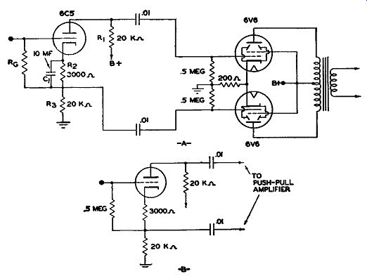
FIG. 10.9. Two alternate phase-inverter circuits.
In Fig. 10.9B, the smaller cathode resistor is left un-by-passed to provide a small amount of negative feedback. This aids the stability of the phase inverter and provides a better high and low frequency response.
Another phase inverter circuit is shown in Fig. 10.10. Here, either V1 or V2 may be separate tubes or else each may be part of a duo-triode. The output of the first triode, V1, is fed to one grid of the push-pull amplifier.
A portion of this voltage, however, is also applied to the grid of the second triode (V2) and the output from this tube applied to the grid of the other push-pull amplifier tube. Since the input and output voltages of V2 differ by 180°, we have the output voltage of V2 differing from the output voltage of V1 by 180°. In this way each grid of the push-pull amplifier receives its voltage in proper phase relationship. Since V2 is used for the sole purpose of taking a portion of the output voltage of V1 and reversing it in phase, it is actually the phase inverter.
The amount of voltage that is fed to the grid of V2 depends upon the ratio of R4 to R3 + R4 and the amplification of V2. Thus, for the voltage amplification at V 2 to be 40, the voltage tapped off at R4 should be 1/40 of the total voltage across R3 + R4.
With this method, each grid of the push pull amplifier tubes receives the same input voltage, and the circuit is balanced. In the present circuit, the ratio of R4 to R3 + R4 should equal 1/40, and substitution of the given values for R3 and R4 , 10,000/410,000, shows this to be approximately true.
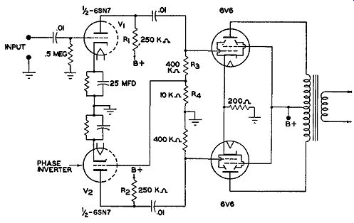
Fig. 10.10. Phase inversion using a separate tube. This arrangement
is sometimes called a paraphase circuit.
Unlike the previous phase inverters, this circuit is capable of fairly high gain. Its greatest disadvantage, however, is the unbalance that occurs when ever the amplification of either triode changes. Both triodes are unrelated and any change that occurs in one section is not automatically compensated for by the other triode. Hence, unless care is taken to measure the characteristics of each tube from time to time (and making compensations there fore), some unbalance will always be present.
Partial compensation for unbalance is obtained by the circuit of Fig. 10.11. A change has been introduced in the grid circuit of the push-pull amplifiers by the insertion of the common resistor, R6 Since R6 is also in the input circuit of the phase-inverter tube, V2, any changes here will also affect this tube's operation. V2 receives its input voltage from R3 and R6 , whereas its output voltage appears across R4 , R5, and R6 . For V1, the output signal is developed across R2 , R3 , and R6.
To understand how the compensation is accomplished, let us suppose that both V1 and V2 are functioning normally. The voltage for tube V3 appears between point A and ground; for tube V4 , between point C and ground.
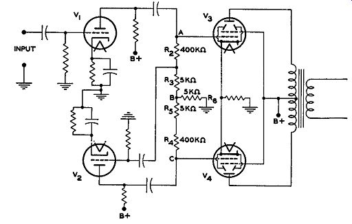
FIG. 10.11. A modified phase inverter to produce automatic balancing.
The voltage present at R6, under normal conditions, is zero because the out-put voltages from V1 and V2 are out of phase and hence cancel across this common resistor. But, now, let us suppose that the amplification of one tube decreases, say, V1. Thus, if point A went positive, say, 8 volts at one instant, point C (with respect to ground) might be 10 volts negative because amplification of V2, Under these circumstances, the net voltage appearing across R6 would not be zero but some small negative value. Since the voltage applied to the grid of V2 is composed (at the moment) of the positive voltage of R3 and the small negative voltage of R6 , the net voltage acting at the grid of V2 is slightly less than it ordinarily would be. As a result, the output voltage of V2 is decreased, counterbalancing the increased amplification of this tube.
Conversely, if V2 should decrease in amplification, a greater voltage would be applied to its grid, giving a correspondingly larger output. With limits, the common resistor R6 tends to maintain a balanced circuit, al though at some sacrifice in overall gain.
Another popular inverter type is the cathode-coupled inverter shown in Fig. 10.12. The first triode, V1A, receives the audio signal from the previous stage across its grid resistor, R1. This signal is amplified and forwarded through 0 1 to the grid of one push-pull amplifier tube. The load resistor for Vu is R2. Since the cathode resistor, R4, is un-by-passed, the signal variations appear in full across it as well as across R2. The grid of V1B is placed at a-c ground potential by C. Thus, the signal variations appearing across R4 are also instrumental in varying the current through V1B and producing an amplified version across plate load resistor R3. From here, the signal is coupled to the grid of the second push-pull amplifier tube.
The two output signals are 180° out-of-phase with each other. A positive increase in signal at the grid of V1A will cause a corresponding increase in voltage at the cathode end of R4. Since the a-c potential of the grid of V1B is fixed (at ground), the positive rise in its cathode voltage is equivalent to a negative increase in grid voltage. Thus, for the same applied voltage, the grid of V 1A is driven in the positive direction while the grid of V 1B goes in the negative direction.
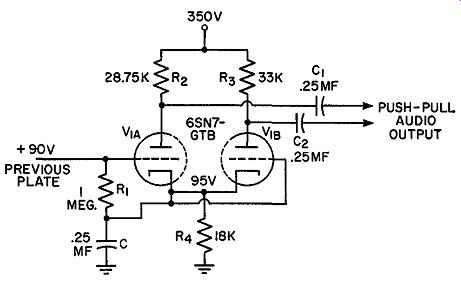
Fig. 10.12. A cathode-coupled phase inverter. (Courtesy Radio & TV
News)
The plate resistors have different values in order to balance the two circuits. Since the cathodes have a fairly high positive voltage, because of the large value of R4, a fairly high positive voltage is required at each grid.
95 volts, positive, is indicated for each cathode; therefore, each grid should be given a positive voltage of 90 volts. This is obtained by direct connection to the plate of the previous stage. The grid of V1B connects directly to the bottom end of R1 in order to obtain the same B+ as the grid of V1A. however, by adding C at the bottom of R1 we are able to keep the grid of V1B at a-c ground.
The cathode-coupled inverter possesses good balance at both high and low frequencies. It is also exceedingly stable because of the large amount of degeneration used. It does not, however, provide any gain and, in this sense, is not as good as either of the previous inverters. The addition of an extra amplifier ahead of the stage will compensate for this.
Negative Feedback. The beneficial effects of feeding back some voltage which is out of phase with the input voltage was mentioned briefly above in connection with phase inverters. Actually in the case of Fig. 10.7, the de generation ( or negative feedback, as it is known) was unintentional. It was necessary to leave R2 unby-passed in order that the alternating voltage developed across it could be transferred to the next stage. However, in many amplifiers, the negative feedback is purposely introduced. Its advantages are:
1. Improvement of the frequency response of the amplifier.
2. Decrease in distortion in an amount depending upon the percentage of voltage fed back.
3. Increased stability, with less tendency for regeneration (whistles or howls) to appear.
It is true, of course, that these advantages are not obtained without a loss-in this case, gain. For, as the degree of negative feedback increases, the gain of an amplifier decreases. However, for most amplifiers, especially those used in radio receivers and small amplifiers, the amount of available gain exceeds the need, and a slight loss for the advantages noted above is voltage well spent.
In negative feedback, a certain pro portion of the output voltage is fed back to a previous stage in opposition to the input voltage that is present at this point.
--- The circuit in Fig. 10.13 illustrates the principle. R1 and R2 form a voltage divider across the output of V1 -- Through the connection from point A to point B, a portion of the audio voltage that is developed at RL is fed back to the grid circuit of V1. Now let us determine whether the voltage fed back is in phase opposition to the incoming voltage appearing across R2.
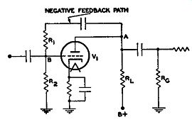
Fig. 10.13. A simple negative feedback circuit. R1 and R2 form a voltage-divider
network across R1.
If the incoming signal to V1 at any instant is going in the positive direction, then the voltage at point A is going negative. This action is due to the increased current through the tube, resulting in a greater voltage drop across RL, leaving the top end (point A) more negative (or less positive because of the increased voltage drop in RL) than it was before the application of the signal. By connecting points A and B together, the voltage from RL (EL) will cancel part of the positive incoming audio voltage at point B. This cancellation is the essential principle of negative feedback. When the incoming signal is strong, more voltage is fed back from A to B and a greater cancellation occurs. With a weak signal, the opposition of the feed back voltage is correspondingly reduced. Thus, the negative feedback voltage acts to maintain a constant output. Again, if distortion is introduced between points B and A, the voltage transferred back will contain this distortion. However, because the voltage fed back from A to point B is opposite in phase to the signal passing through V1 , the feedback voltage will introduce this distortion in a manner opposite to that produced by the tube.
When the signal, with this reverse distortion, passes through the tube, the impact of the tube distortion is partially nullified. The result-a decrease in the overall distortion as seen in the output.
The amount of feedback in the circuit of Fig. 10.13 is determined by the ratio of R2 to R1 + R2. (R1 + R2 parallel RL and the output is developed across them.) This voltage is divided between them in direct proportion to their relative resistances, with the larger resistor obtaining a larger percent age of the voltage. If R2 is large, a greater percentage of voltage will be transferred to point B. This, in turn, will lower the gain considerably. Generally a compromise is reached, where the gain is still appreciable but sufficient feedback is developed to afford good stability with low distortion.
One very simple form of negative feedback is obtained by removing the-- cathode by-pass capacitor (see Fig. 10.14). The a-c portion of the plate current must now flow through the cathode resistor Rk instead of being by-passed. As a result, an alternating voltage is developed across Rk which opposes the input signal. To illustrate, suppose the grid of V1 is made positive by an incoming signal. The plate current through V1 will increase, increasing the voltage drop across Rk with the polarity as noted. However, the voltage at the grid that caused the increased flow of current through the tube is the grid-to-cathode voltage.
Since, in this instance, the cathode becomes more positive, part of the positive signal voltage rise at the grid is counterbalanced by the positive voltage rise at the cathode.
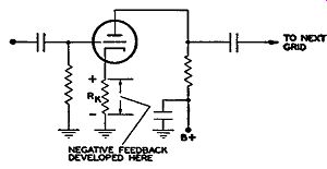
FIG. 10.14. Negative feedback obtained from an unby-passed cathode resistor.
There are many other possible arrangements and several of the more common methods are shown in Fig. 10.15. In each instance the opposition of the voltage being fed back may be noted by following the procedure out lined above. Feedback may occur from the plate of one stage to its grid, or it may extend over several stages. Whatever the method, care must be taken to see that the feedback is degenerative, not regenerative. Regenerative feedback means voltage fed back in phase, not out of phase, and under these conditions oscillations will occur.
Output Stages. Mention has already been made at the start of this Section of the advantages of push-pull operation and, for this reason, most high fidelity amplifiers use this form of circuit. However, before we ex-amine some of the most popular push-pull circuit arrangements, it should be noted that single-ended stages are used also, particularly in table-model receivers where the output power requirements are quite low. For example, the audio amplifier section of one such FM receiver is shown in Fig. 10.16.
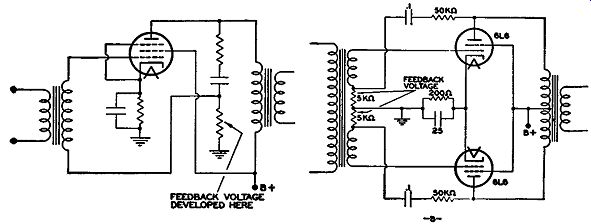
FIG. 10.15. Two additional methods for obtaining negative feedback.
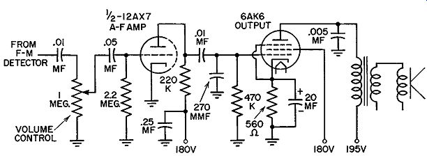
FIG. 10.16. The audio amplifier section of a table-model FM receiver.
The sound output of the preceding ratio detector is fed through a volume control to one triode section of a 12AX7. This is a voltage amplifier. The signal next is applied to a 6AK6 pentode output stage and, from here, to an output transformer and a 5-inch speaker. In essentially all respects, this amplifier section is equivalent to those found in most AM radio receivers.
Push-pull output circuits fall into two general categories, those using triodes and those using pentodes or tetrodes. (The latter two tube types are grouped together because they function in essentially the same manner and provide similar results.) In the early days of high fidelity, triodes or pentodes and tetrodes connected as triodes were used most extensively be cause they provided the best results from a distortion standpoint. Then, to reduce whatever distortion did appear, negative feedback was inserted.
The famous Williamson amplifier used such an arrangement, as shown in Fig. 10.17. The input signal is amplified by one triode section (F1A) of a 6SN7GT. The signal is then directly-coupled to the second triode, V1B, where two oppositely-phased voltages are developed to drive V2. Thus V1B is a split-load phase inverter. V2 serves as a driver, to strengthen the signal it receives to drive output tubes V3 and V4. These two tubes are beam power tetrodes connected as triodes. The signal is then fed to the output trans former and, from here, to the loudspeaker.
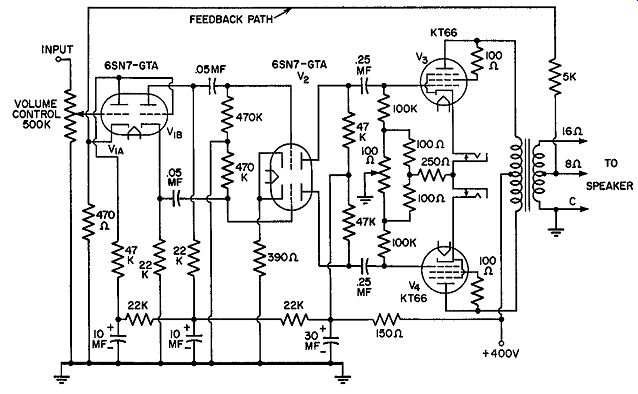
Fig. 10.17. The Williamson amplifier in which the two beam-power tetrode
output tubes, V3 and V4, are connected as triodes.
Negative feedback, to stabilize the system and reduce distortion, is employed between the secondary of the output transformer and the cathode of V1A. As a further aid to the minimization of distortion, the two output amplifier circuits are balanced by a 100-ohm potentiometer. This is in the grid circuits of V3 and V4; it is adjusted correctly when both tubes draw the same cathode current with no applied signal.
A tetrode or pentode, connected as a triode, requires less driving power for a specified output than does a triode. However, a tetrode or pentode does introduce a greater amount of distortion. A configuration which combines high power sensitivity with low distortion is the Ultra-Linear arrangement shown in Fig. 10.18. The plates of the output tubes are connected to opposite ends of the primary winding of the output transformer, as before. However, special taps are available on the winding for the screen grid of each tube. This has the effect of providing some negative feedback to the screen grid circuit which straightens out the characteristic curves of these tetrode (or pentode) tubes. The result is very low distortion with good power sensitivity.
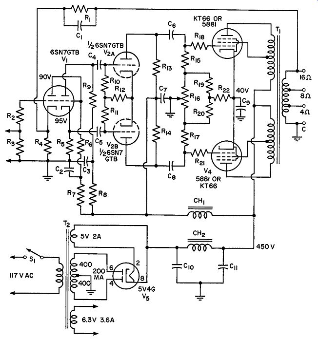
Fig. 10.18. A power amplifier in which the output tubes (V3 and V4 )
are employed in an ultra-linear arrangement.
Still another output power amplifier circuit that has received attention is the cathode feedback circuit shown in Fig. 10.19. A special winding is added to the output transformer and the cathode of each tube is connected to one end of this winding. This arrangement has excellent fidelity characteristics (i.e., low distortion), but it requires a considerable amount of driving voltage because of the cathode degeneration. In this sense, it is quite similar to the cathode follower, where the gain is low.
Where extremely high output power is desired, on the order of 60 watts or more, it is common practice to parallel the output amplifiers. Generally, two tubes in parallel for each half of the output amplifier suffice for most high power requirements. However, if more power is needed, additional tubes can be added.
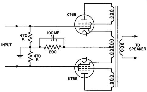
Fig. 10.19. A push-pull output amplifier using cathode feedback.
Most push-pull amplifiers are conservatively operated as Class A or Class AB1 . This results in low distortion. True Class-B operation requires more driving power and introduces stricter design requirements that can raise the cost of the unit. Consequently, Class-B operation is not used as often.
Cathode Followers. It is common practice in modern high-fidelity receivers to have the tuner separate from the audio amplifier. The tuner, whether it be a combination AM, FM unit or designed for AM or FM alone, receives the incoming signal, amplifies it, and detects it. After per haps one stage of audio amplification, the signal is ready to be applied to the audio amplifier where it will be strengthened sufficiently to drive the loudspeakers.
In order to transfer the signal from the tuner to the amplifier, a shielded coaxial cable is employed. This cable has a fairly low impedance, of the order of 600 ohms, and to shunt the normal plate load resistor of an amplifier with so low an impedance would not only reduce the output voltage to a very small value, but it would also cause considerable signal distortion.
Much more useful in matching the cable's impedance is the special amplifier stage known as a cathode follower. The basic form of this circuit is shown in Fig. 10.20. The load resistor is removed from the plate circuit and shifted to the cathode branch. No by-pass capacitor is used and any applied audio voltages between grid and cathode will appear across R,,.
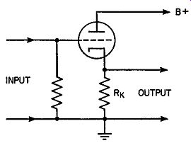
Fig. 10.20. The basic cathode follower.
The output signal can then be taken from this point.
Since the cathode resistor is unby passed, considerable degeneration will occur. Furthermore, the phase of the voltage across Rk is the same as the signal phase at the grid. For example, if a positive-going signal is applied to the INPUT grid, the rise in plate current will produce a greater voltage drop across Rk, making the cathode more positive. Likewise, a negative-going voltage at the grid will reduce the plate current, decreasing the voltage drop across Rk. This will make the cathode less positive or, what is the same thing, more negative.
Thus, the voltage across the cathode resistor "follows" the grid and this is the reason why this circuit is called a "cathode follower."
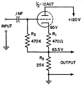
Fig. 10.21. A modification of the cathode follower of Fig. 10.20. The
voltages shown are with respect to ground.
The gain of a cathode follower is normally on the order of 0.9. This means there is a slight loss, due to the large amount of degeneration or negative feedback. The degeneration is also responsible for the low output impedance of the stage. It is this low output impedance which makes it possible to use a coaxial cable between the cathode follower and the power amplifier.
A modification of the cathode follower, which is used more frequently than the basic arrangement of Fig. 10.20, is shown in Fig. 10.21. This possesses a separate bias resistor R1 which establishes the operating voltage between grid and cathode. The grid input resistor, R3, is then connected between the grid and the bottom end of R1. With a large resistor in the cathode circuit, the cathode voltage will be correspondingly high-here on the order of -65 volts. If R3 is returned to ground, the grid would see a negative bias of -65 volts, sufficient to cut the tube off. (Actually, the tube could not cut itself off, for then the cathode voltage would disappear. However, enough current would flow to bring the tube close to cutoff.) All this is avoided by returning R3 to the bottom end of R1. Now the grid-to-cathode voltage is -1.5 volts and the d-c voltage drop across R2 does not affect this bias. However, since R2 is unby-passed, it still produces the cathode follower action.
Preamplifiers. Before we leave the subject of audio amplifiers, mention should be made of preamplifiers. These are specially designed amplifiers which take the exceedingly small voltages developed by modern magnetic cartridges such as are used in record players and amplify them so that they can be fed into the input of a power amplifier.
1. The average voltage obtained from a magnetic cartridge is on the order of 15 to 20 millivolts. This voltage is too small to drive a power amplifier.
The word "special" is emphasized in connection with preamplifiers be cause of the precautions necessary to minimize hum and resistor and tube noise ( described earlier). With the desired signal possessing a very small amplitude, any hum or noise which, in ordinary amplifiers, could be ignored, must be carefully avoided in preamplifiers. Otherwise, the amplification accorded the signal will serve equally to strengthen the hum or noise and provide an input signal to the main amplifier having a strong hum or noise background.
To reduce tube hum, the filament has a spiral construction in which the magnetic field ordinarily set up by the current heating the filament is reduced to as low a value as possible. Additional precautions are also taken to prevent current leakage from filament to cathode, another source of hum trouble. So important is the need to minimize hum in the preamplifier that many designers use d-c to heat the filaments instead of a-c. The required current can be obtained from a separate power supply or by utilizing the cathode currents flowing through the power output amplifier.
Noise arises from the current flowing in the preamplifier tubes and from the grid and plate resistors used with these tubes. Special construction will also reduce tube internal noise. Resistor noise is reduced by using de posited film resistors and noninductive wire-wound resistors. These produce considerably less noise than composition resistors of the same rating.
The circuit diagram of a two-stage preamplifier is shown in Fig. 10.22.
It is similar in design to a conventional audio voltage amplifier, incorporating, however, the low hum and low noise features mentioned previously.
[ 1. By power amplifier, we refer here not solely to the final stage of an audio amplifier system, but the entire system, such as that shown in Fig. 10.17]
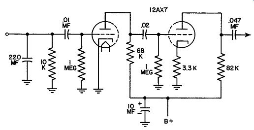
Fig. 10.22. A record player preamplifier.
The 12AX7, for example, is specially designed to possess low noise and low hum. Also, the resistors are carefully selected for their low noise qualities.
Most preamplifiers also incorporate an equalization network, either between the two stages or between the last stage and the output of the section. The same preamplifier (Fig. 10.22), with a number of equalizing circuits, is shown in Fig. 10.23. Five equalizing networks are shown, and the desired one can be selected by a special 5-position switch.
Equalizing circuits are needed to counterbalance the inverse process which is applied to records when they are manufactured. For example, when a record groove is cut for a low frequency sound, the applied voltage from the microphone (or its amplifiers) is reduced in order to avoid cutting too wide a groove. This is called de-emphasizing the low frequencies. On the other hand, frequencies above 1000 cycles are given additional amplification—i.e., pre-emphasized--in order to overcome the surface noise which is present in the record. At the amplifier, on playback, these signals must be returned to their proper relative amplitudes. This is the purpose of the equalizing networks. They are designed to de-emphasize the high frequencies and emphasize the low frequencies. When properly carried out, the net result is an exact reproduction of the original audio signals fed to the recording system.
Five different equalizing networks are used in the preamplifier in Fig. 10.23. Prior to 1953, there was no general agreement on the amount of de emphasis and pre-emphasis to employ when cutting a record. Each record manufacturer set his own standard. Thus, Columbia Records had one re cording and playback curve, RCA utilized another, etc. To develop the proper sounds from these records, each had to be played back with the correct equalization network. In 1953, however, agreement was reached by the major record manufacturers on a standard curve and, as this was done under the auspices of the Record Industry Association of America, Inc., the curve is now known as the RIAA curve.
In the preamplifier of Fig. 10.23, RIAA equalization is obtained with the selector switch in the third position. Since many of the older records are still in circulation, equalizing networks for the more popular of these are also included. These are: LP, XAB, and AES. One position, too, is provided for European records, as these require still a different equalization network.
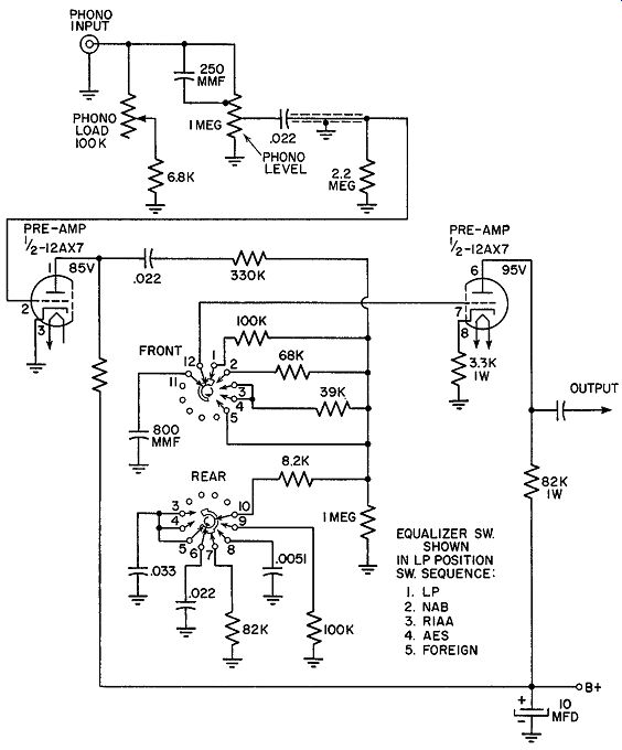
Fig. 10.23 A commercial preamplifier with an equalizing network. (Courtesy
H. W. Sams & Co.)
A comparison of these different equalization curves are shown in Fig. 10.24. These are the curves of the playback amplifier equalization networks where the low frequencies are emphasized and the high frequencies are de emphasized. In the record-cutting equipment, the inverse equalization characteristic would be applied. That is, the low frequencies would be de-emphasized and the high frequencies emphasized.
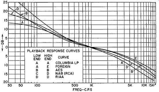
Fig. 10.24. Five equalization curves that have been used by record manufacturers.
The standard curve, at present, is the RIAA ( curve D). ( Courtesy Radio
Electronics)
Tone Control Circuits. It is due to a recognition of the variation in individual tastes plus the fact that radios are used in widely differing locations that tone controls are incorporated into a large number of sets. Tone control permits the listener to vary the amplification applied to a range of frequencies and in this way cause a definite accentuation or boosting within this range. For the reception of music, for example, many listeners prefer to turn their tone control to the point where the bass frequencies predominate. For speech, the adjustment is made toward the higher frequencies.
Whatever the preference, we are more interested in this discussion as to how tone control is electrically achieved rather than why a certain tone is preferred.
Tone-control systems are essentially of two types. In one system, the apparent accentuation of one range of frequencies is achieved not by an actual boost within this range but by decreasing the strength of the other frequencies present. For example, to raise the level of bass frequencies, many manufacturers provide an adjustment which will accomplish this boost in a relative manner, by decreasing the intensity of the treble frequencies.
The effect of the high frequency decrease upon the listener is as though there had been an accentuation of the bass tones. The second system involves an actual boosting of the frequencies that we desire to accentuate.
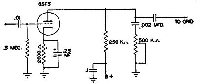
Fig. 10.25. A simple bass-boost tone control. The variation of control
is accomplished with the 500,000-ohm potentiometer, but the entire tone
control circuit includes also the 0.002-mf capacitor.
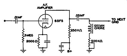
Fig. 10.26. A simple treble tone control.
Simple Bass-Boost Control. A simple tone control that is found in many sets is shown in Fig. 10.25. It is placed in the plate circuit of one of the audio amplifiers and functions through its ability to decrease the relative strength of the high frequencies that are permitted to reach the speaker. When the center arm of the resistor is at the end nearest the capacitor, the decrease of the high frequencies is maximum because only the capacitor is opposing their passage around the plate circuit. At these times the bass output will seem strongest; moving the center arm to the opposite end of the resistor permits a greater percentage of the highs to reach the output because the by-passing path's resistance has been increased.
Treble Control. The opposite effect can be achieved by replacing the series capacitor of Fig. 10.25 with a series choke coil, as shown in Fig. 10.26.
Now we have a path for the low frequencies to be shunted away from the output. When the center arm is at the end of the resistor nearest the coil, the maximum shunting effect is imposed on the low frequencies. The position would correspond to greatest treble output from the set. When the center arm is at the opposite end of the resistor, the opposition to the lows has increased, providing more frequencies from this range for the output.
If we wish to combine both circuits, obtaining a more flexible control, we have the arrangement of Fig. 10.27. This unit is particularly useful at low volume levels because it tends to provide a more uniform response over the entire audio range. It was noted from the response curves of the ear in Fig. 10.7 that, as the volume is decreased, the high and low frequencies de crease more rapidly than the middle-range frequencies. In the control of Fig. 10.27, the middle frequencies are attenuated more than those at either end of the audio range. The overall result is a more uniform distribution.
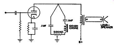
Fig. 10.27. A combination "treble-bass" tone control.
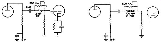
Fig. 10.28A. A series treble tone control. Fig. 10.28B. A series bass
boost tone control.
Instead of placing the tone control in shunt across the circuit, it is also possible to place it in a series branch. For low frequency attenuation, the circuit of Fig. 10.28A is possible. The low frequencies lose more voltage across C1 than the higher frequencies. Hence, when R1 is completely in the circuit, the greatest amount of loss occurs at the low frequencies. By gradually shunting out a part of R1, we can raise the intensity of the lows at the output. As a treble attenuator, the capacitor can be replaced by a choke (see Fig. 10.28B).
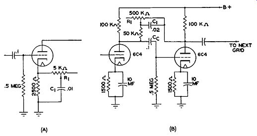
FIG. 10.29. Two common methods of applying negative feedback to obtain
tone control.
Tone Control by Inverse Feedback. Tone variation can be also accomplished by inverse or negative feedback methods. Two popular methods are shown in Fig. 10.29. In Fig. 10.29A, negative feedback effect is incorporated in the cathode leg of the tube. R1 and C1 , in series, provide the degenerative effect. The value of C1 determines the frequencies at which the effect first becomes noticeable. If C1 is small in value, the decrease in output occurs at the middle and low frequencies; if C1 is large, the output decreases only for the very low frequencies. The whole operation of this network depends upon the fact that if the cathode bias resistor is not adequately by-passed, the voltage across it will vary and tend to counteract the effect of the input voltage. When C1 is small, only the higher frequencies are readily by-passed, the middle and lower frequencies producing a variable drop across C1 because of the substantial impedance offered them by the capacitor. The variable cathode bias (for the frequencies mentioned) will partly counteract input voltages of the same frequencies. The result is that the higher frequencies remain untouched and appear more strongly at the loudspeaker. As C1 is made larger in value, its opposition to even the lower frequencies decreases. Hence, these, too, pass through un diminished. The inclusion of the additional frequencies lessens the aural effect of the highs, and the tone becomes deeper. R1 is inserted to provide a variable adjustment.
Another approach to the problem of negative feedback tone control is the plate-to-plate connection illustrated in Fig. 10.29B. Actually, what we do here is to feed back a voltage from the plate of the second 6C4 to the grid of the same tube. We use the plate-to-plate connection to keep the positive B+ voltage of the 6C4 from reaching its grid. Cc isolates the voltage from the grid. In the circuit, C1 and R1 combine to regulate the high frequency voltage that is fed back from the plate to the grid. Since the high frequencies return out of phase, they decrease other incoming high frequencies, permitting the lows to dominate at the output. The position of the center arm of R1 determines how much high frequency degeneration occurs.
In all of these circuits, it is to be understood that no network permits one range of frequencies to pass, excluding all others. It is merely that one range of frequencies is offered less opposition than other frequencies and, hence, a proportionately greater amount of voltage from this range passes through.
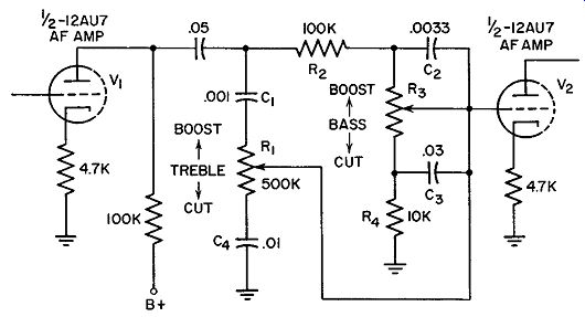
Fig. 10.30. A continuously variable tone control.
Continuously Variable Tone Controls. All of the preceding tone control circuits have been so designed that, in order to obtain either a high or low frequency output sound, the opposite range of frequencies is attenuated. The circuits have the advantages of economy in construction and simplicity of design. Much more complex are those arrangements whereby a boost or increase is given to the section of frequencies we desire to accentuate. A typical circuit is shown in Fig. 10.30. It is capable of independently boosting or attenuating both the high and low frequencies. This is graphically illustrated by the curves shown in Fig. 10.31. At the low-frequency end of the graph, the upper curve demonstrates the effect of bass boost.
This is 16 db at 30 cycles. The lower curve at this end is the bass cut and it reaches a value of 15 db. At the right-hand side of the graph, the extent of the treble boost is revealed by the upper curve and is seen to reach a value of 16 db at 20,000 cycles. Treble cut, at this frequency, is 17 db.
The action at intermediate frequencies, between 30 cycles and 20,000 cycles, is indicated by these curves.
In the circuit, R2, R3, R4, C2, and C3 form the bass boost and cut circuit. R3 is the variable front-panel adjustment. In its maximum clock-wise position, the bass output is greatest; in its maximum counter-clockwise position, the bass output is lowest. The taper on the control is such that, in its mid-position, the resistance between the arm and the lower end of the control represents only about 10% of the total resistance of the potentiometer. This means that any medium frequency signal passing through will be reduced in the ratio of 10 to 1. This is also true at the high frequencies, when C2 and Cs effectively short out Rs, because then R2 and R4 possess the same 10 to 1 ratio.
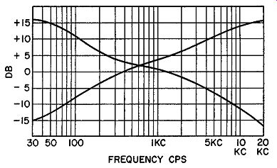
Fig. 10.31. Curves showing the compensating effect of the bass and treble
tone controls of Fig. 10.30.
Note that the capacitance values of Cs and 0 2 are also proportioned in the 10 to 1 ratio to insure that this division is maintained at all frequencies with the arm of Rs in the center position.
Consider, now, what happens when the arm of Rs is moved up. This is the bass boost position. C2 is shorted out. For the high audio frequencies, Cs presents a very low impedance, and any signal coming from the previous stage divides between R2 and R4. Since R4 has a resistance one-tenth that of R2, the next stage (V 2) receives one-tenth of the total signal.
As the signal frequency decreases, the impedance of Cs rises, applying more and more voltage to the grid of V2. At 30 cycles, the impedance of Cs is so high that V2 receives nearly 9/10 of the applied signal. This rep resents a boost over the center setting of the bass control.
When the arm of Rs is turned to its maximum counter-clockwise position, Cs is shorted out. High audio frequencies pass through C2 readily and divide between R2 and R4 in the ratio of 10 to 1. As the frequency decreases, the impedance of C2 rises and this places a greater impedance in the path of the signal before it reaches R4. Hence, less voltage develops across R4 , and less reaches V2, At 30 cycles, the voltage reaching V2 is reduced 15 db below its value when the arm of Rs is in mid-position.
The treble control circuit consists of C1, C4, and R1. The potentiometer, R1, has the same type of taper as R3 so that, when it is in mid-position, only 10% of the 500,000 ohms is between the arm and C4. In this position, only 10% of all the high frequencies applied to this network reach V2. When the arm is turned to the top of R1 , considerably more of the high frequency signal reaches V2. By the same token, when the arm is turned to the bottom of R1, very little of this signal reaches V2, This is the treble cut position.
There are other versions of this control, but with the help of the fore going explanation, there should be little difficulty in understanding their operation.
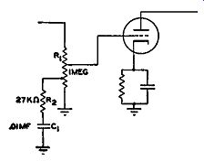
Fig. 10.32. A fixed-tone compensation circuit.
Automatic Tone Compensation. Before we leave the subject of tone controls, there is one commonly used network that provides a fixed amount of tone compensation at the volume control. In Fig. 10.32 a series resistor and capacitor are tapped across the lower section of the volume control. When the volume is turned up high, the tone compensation network has no appreciable effect. At low volume levels, however, when the center arm of R1 is near the lower end of the volume control, R2 and C1 become effective. Their purpose is to attenuate somewhat the amount of middle and high frequencies that reach the succeeding amplifiers. The need for the compensation is due to the fact that at low volume levels the human ear is least sensitive to the low frequencies. Partially to offset this limitation, some of the higher frequency voltage is by-passed by C1 and R2. The aural effect is an apparent increase in low frequencies at low volume.
Many high-fidelity amplifiers extend the range of tone compensation by inserting several compensation networks, each designed for a different level of sound. The circuits are brought into the system by a special selector switch, usually labeled a "Loudness" control. This is discussed more fully in Section 12.
EXAM
1. State briefly what factors must be taken into consideration in any discussion of high fidelity.
2. How do the properties of the human ear affect high fidelity? Describe some of these properties.
3. What have radio manufacturers done in recognition of the frequency and loudness characteristics of the human ear?
4. Describe what is meant by "frequency balance."
5. Draw the diagram of a frequency-dividing network designed to feed signals to special high and low frequency speakers.
6. What are the advantages of push-pull amplifiers over single-ended amplifiers?
7. Must push-pull amplifiers always be transformer-coupled to the previous amplifiers? Explain.
8. Draw the circuit diagram of a push-pull amplifier.
9. What is a phase inverter? Why is it useful?
10. Draw the circuit diagram of a single phase inverter tube driving a push-pull amplifier.
11. Why can a single tube be used to provide two out-of-phase voltages?
12. What are the advantages and disadvantages of using a single tube to drive a push-pull amplifier?
13. Draw the circuit schematic of a single amplifier and a separate phase inverter driving a push-pull amplifier.
14. What is negative feedback?
15. What are the advantages of negative feedback?
16. Describe several methods for achieving negative feedback.
17. What precautions must be observed when using negative feedback?
18. What type of tone control is used on most radio receivers? Explain how it functions.
19. Draw the diagram of an audio amplifier containing a simple bass-boost tone control.
20. Illustrate the differences between bass and treble tone controls.
21. Explain how negative feedback can be used to obtain tone control.
22. Draw the diagram of a circuit using negative feedback to obtain tone control.
23. Explain how the circuit of Fig. 10.30 operates.
24. What is automatic tone compensation? Why is it used? How is it achieved?
25. What is a cathode follower? Where would it be found in audio equipment.
26. Illustrate, with simple diagrams, three different types of audio output circuits.
27. Explain the advantages and disadvantages of the following output amplifiers: triodes; tetrodes connected as triodes; tetrodes with cathode feedback.
28. When are preamplifiers required? What precautions must be taken when preamplifiers are designed?
29. What is meant by equalization? Where is it generally applied in audio equipment?
+++++++++++