IN professional recording work, there are 2 principal reasons for the use of equalizer circuits. First, discs cut at 33 1/3 r.p.m. lose some high-frequency response as the stylus nears the center of the record. Second, the recorder may want special response curves, such as Orthacoustic, Columbia Transcription and NAB Standard. In amateur and semiprofessional work 2 more reasons for equalization often appear. If the response of the cutter is not linear, some compensation can be made. If a crystal cutter is used, special connection circuits must be used, and its response will depend on how it is fed by the amplifier.
Frequency-response control for playback of finished discs is discussed in Section 13.
The recording amplifier system must have a flat frequency response.
If there are peaks or if the amplifier curve drops off excessively on the high- or low-frequency end, equalization is not the cure. It is easy to build a flat amplifier (50 to at least 8,000 cycles) if proper attention is paid to high-quality components and circuit wiring. If the amplifier does not turn out well, do not insert equalizers to correct the original frequency response of the amplifier. Experimentation with the amplifier is indicated.
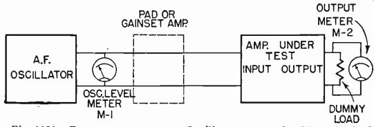
Fig. 1101--Frequency run setup. Oscillator output should not be high
enough to overload the initial amplifier stages, but sufficient to give
a reading on meter M-1.
Making Frequency Runs
It is a good idea to make a frequency run on the amplifying system before equalization is attempted. For those who are unfamiliar with this procedure, the following detailed outline is given. This method of determining response curves is valuable in any audio work and will be necessary in equalizing the system.
The materials needed are :
1. An a.f. test oscillator with frequency variable from 50 to 10,000 cycles. Output voltage should be sufficient to be readable on a meter, and output impedance should be 5,000 ohms or higher. There should also be a selection of low impedances. Any commercial audio test oscillator will suffice.
2. Unless the oscillator has a built-in output meter or is of the constant-output, R-C type, a meter should be provided. Oscillator output must be kept constant at all frequencies.
3. A dummy load resistor of the same value as the output impedance of the amplifier system, with a wattage equal to the maximum capability of the amplifier.
4. A high-resistance (1,000 ohms-per-volt or better) a.c. voltmeter to measure amplifier output. A vacuum-tube voltmeter or one using a crystal rather than a dry-disc rectifier is ideal because it will not have frequency discrimination in the audio range.
5. Pencils and plenty of paper.
6. A good supply of graph paper (semi-log paper with 3 cycles by 70 divisions).
Connect the oscillator to one of the inputs of the amplifier system.
Set its output high enough so that some indication can be seen on the amplifier voltmeter. Usually, a vacuum-tube voltmeter must be used to show oscillator output when impedance is high because the low resistance of ordinary meters interferes with operation of the test setup.
Disconnect the amplifier output from the cutter and substitute a dummy load resistor of the same impedance as the amplifier output.
Across the dummy load resistor connect the output meter. Now the frequency run can be made, as shown in the following steps:
1. Adjust the oscillator to a reference frequency, such as 1,000 cycles.
2. Adjust amplifier and oscillator gain controls so that the amplifier output meter indicates some convenient value near center scale. Be sure that the oscillator output is not so high as to overload the initial amplifier stages, and that oscillator output is sufficient to give a reading on the meter across its terminals, if one is used. If a low7impedance, high-gain input is being fed, a pad may be inserted between oscillator and amplifier to reduce actual input while still putting out enough level to actuate the oscillator output meter. The setup is shown in Fig. 1101.
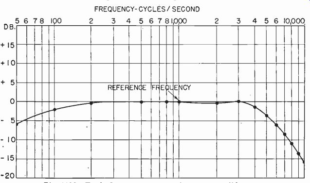
Fig. 1102-Typical response curve of a poor amplifier.
3. Make a note of both meter readings. For all future steps, adjust only oscillator output to keep the reading of M-1 (Fig. 1101) at this same point. Don't touch amplifier gain control during these steps. This is most important.
4. Adjust the oscillator to each of the following frequencies, adjusting the oscillator output to keep it constant and making a note of the reading on the amplifier output meter M-2: 50, 100, 200, 500, 800, 1,000, 2,000, 3,000, 4,000, 5,000, 6,000, 7,000, 8,000, 9,000, and 10,000 cycles. The voltage output of the amplifier for each frequency should be tabulated on a sheet of paper.
5. Calibrate a sheet of the graph paper as shown in Fig. 1102.
The horizontal lines represent decibels and the vertical lines represent frequency. Select a horizontal line in the center of the sheet and mark it 0 db. In the left margin, mark the lines above plus and below minus.
6. Make a pencil dot at the point where zero db intersects the chosen reference frequency (1,000 cycles in Fig. 1102).
7. On a separate sheet of ordinary paper, calculate the decibel relationship between the output at the reference frequency and that at 50 cycles. To do this, divide the larger voltage by the smaller. For instance, if output at the reference frequency 1,000 cycles was 6 volts and at 50 cycles was 3, dividing the 6 by 3 (6/3) gives 2. This is the voltage ratio of 50-cycle output to 1,000-cycle output. To convert to decibels, look up 2 in the column headed "Voltage Ratio" in Table 11-1. Read decibels under the column headed "Decibel Gain or Loss." In this case, a voltage ratio of 2 equals a decibel gain or loss of 6. Since 50-cycle output was lower than 1,000-cycle output, this must be a 6 db loss. Make a dot on the graph where 50 cycles inter sects with minus 6 db.
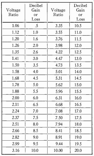
Table 11-1--Abbreviated decibel table.
Voltage ratios are those found in step 7 in text.
8. Follow this same procedure for each of the other frequencies used in the test. For instance, in Fig. 1102, voltage output at 3,000 cycles was the same as that at 1,000 cycles.
The dot at 3,000 coincides with the zero line. At 10,000 cycles output was only 1 volt. Dividing 6 (output at the reference frequency) by 1 gives 6. The nearest figure to that in Table 11-1 is 5.96. The equivalent db is 15.5 The 10,000-cycle dot coincides with the line for minus 15.5 db.
NOTE : Do not interpolate with this table. Values are not linear and results will be incorrect. Decimal accuracy is not necessary.
9. After all the dots are made and rechecked, join them with a solid line.
Fig. 1103-Light pattern of disc cut by a very high quality cutter, showing
an almost perfect frequency response.
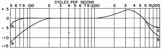
Fig. 1104--Output of standard frequency record (curve A) and output
of recorded test disc (curve B).
Interpreting the Curve
The curve of Fig. 1102 shows the frequency response of an amplifier, obtained as shown above. An inspection quickly shows that the high-frequency response is far from satisfactory. For good results, there should not be much drop-off up to 8,000 cycles. Eleven db, as shown here, is far too much. The unit should be reworked to eliminate stray capacitances in the wiring. Perhaps too much shielded wire has been used. Perhaps circuit design is faulty. After modification, this whole process of taking a frequency run should be repeated. When the curve is practically flat (within 2 db) from 50 to at least 8,000 cycles, the amplifier can be called suitable. For professional work 1.5 db, or better, from 30 to at least 10,000 cycles is required.
Using Magnetic Cutters
If a magnetic cutter is used, the actual recorded frequency curve to be achieved will be modified constant velocity, or some variation of that characteristic. There are 2 methods in common use for measuring the frequency response of a disc cut in this way.
The first and quickest is the light method:
1. Connect the audio oscillator to the amplifier input as before, with provisions for keeping its output level constant.
2. Cut a disc at 78 r.p.m., recording a series of frequencies from 10,000 cycles down to 50 cycles. If the cut is made outside-in, start with the highest frequency ; if it is made in the other direction, start with the lowest. Record each frequency for about 5 seconds, then leave an unmodulated space of about 3 or 4 seconds. Make a careful list of the frequencies to be used.
3. Now hold the finished disc obliquely under a single light source and observe the "Christmas tree" pattern of the cut grooves. Adjust the positions of the disc, light source, and eye until something like the picture of Fig. 1103 is seen.
4. A disc with a practically perfect frequency response will appear like the one in the photo ; the bands from the highest useful frequency down to the turnover frequency will be about the same width. From turnover downward, the bands will gradually become narrower.
This method does not lend itself to very exact measurement, but it is an excellent way to make a quick preliminary check on the high frequencies. From turnover upward, the width of the light band is in direct proportion to the recorded voltage. Measurement can be made with a ruler, and the voltage ratios can be translated into decibel gain or loss, just as in actual voltage measurements. This is not true below turnover.
Incidentally, this check will show almost the exact turnover frequency mechanically built into the cutter.
After a quick look at the "Christmas tree" pattern, more exact measurements can be made to determine the exact equalization required (if any) to correct cutter deficiencies. Procure one of the standard-frequency records on the market. These discs have a series of tones recorded on them with a perfect modified-constant-velocity characteristic similar to Figs. 605, 606 and 1103. Get one such as Columbia #10004-M, with a 500-cycle turnover. We propose to measure cutter response by comparing the records it cuts with the standard-frequency records, so a good playback pickup will be needed, together with a separate amplifier. The pickup-amplifier system should be of good quality. It can be adjusted with the standard-frequency record, according to the instructions in Section 13. Refer to that Section and adjust the playback system before going ahead with the rest of this process.
Assuming that the playback system is reasonably good, play the frequency record on it and make a graph of output, just as shown earlier in this Section. The only difference will be that the tone source is now a record and pickup instead of an a.f. oscillator. Amplifier gain controls, once set, should be left alone during this test. The graph thus made might be like curve A in Fig. 1104. The fact that this curve is not flat shows that the pickup-amplifier arrangement is not quite flat, but this does not matter if we are concerned only with cutter calibration.
Now play, on the same playback system, the frequency record which was made on the new recording machine. Chart its output in the same manner. In both charts, use the 500-cycle turnover frequency as the reference frequency, so that the 500-cycle point on both graphs will coincide on the 0-db line. Plot the curve of the new disc on the same piece of graph paper. Curve B in Fig. 1104 is an example of a new disc.
Now compare the two. In the example, the test-record level at 50 cycles is obviously 7.5 db lower than that of the standard disc. At 10,000 cycles it is 4.5 db lower. Curve A, representing the standard record, is the ideal, and we can easily draw a new graph showing the differences between our disc and the ideal. Fig. 1105 shows the difference in the example chosen. As we have pointed out, the 50-cycle test record level was 7.5 db lower than that of the standard record ; therefore, in curve A of Fig. 1105 the 50-cycle level is shown as--7.5 db, and so on.
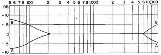
Fig. 1105-Difference between test disc and ideal (curve A). Curve B
shows equalization necessary.
Now insert enough equalization to counterbalance exactly the drop off on each end of the frequency range. In other words, use an equalizer that will raise the 50-cycle level of the recording system by exactly 7.5 db, etc. The work the equalizer must do is shown in curve B of Fig. 1105. The graph makes equalizer selection easy; thus in the example it is obvious that a bass booster is needed. For anything but high-fidelity professional work, we would probably leave the high end alone, since the drop-off of 3 db at 8,000 cycles is not serious.
Choice of Equalizer Circuit
The next step is to choose the equalizer circuit. The best practice is to build into the amplifier a versatile equalizer allowing either boost or attenuation of both highs and lows separately, such as the one shown later in this Section; but if space is left on the chassis, the equalizer may be selected after the amplifier has been built.
Most high-quality professional installations do not include equalization within the recording amplifier. Invariably, in such systems, the setup shown in Fig. 904 is used. Since high-fidelity, expensive cutters are incorporated, equalization to compensate for cutter deficiencies is unnecessary. What equalization is needed for other purposes is usually placed in the 500-600-ohm line between console and recording amplifier. However, in less elaborate installations, it is permissible to have the equalizers within the recording amplifier. Several equalizers are shown at the end of this Section.
After the equalizer has been selected and installed, refer to the original graph showing the final response of the amplifier without equalization. Replace the cutter with the dummy resistor, connect the a.f. oscillator to the recording amplifier input, and make new frequency runs.
The object now will be to adjust the equalizer to obtain an amplifier response which will be the same as before, but with the addition of the necessary equalization. For example, if the amplifier was originally flat from 50 to 10,000 cycles, the equalizer now should be adjusted so that the response looks like curve B in Fig. 1105. Whatever the amplifier response was, the 50-cycle response should now be raised by 7.5 decibels (in our example), and so on.
Next, reconnect the cutter and make a new test record. Compare this again with the standard disc. If the complete procedure has been followed faithfully and accurately, the two should be very similar. If not, make a new graph of the difference and re-equalize.
Setting the frequency response of a recording system is not a quick, offhand operation. It is, on the contrary, a job requiring patience, time, and attention to detail. It is very unlikely that the disc cut will match precisely the characteristics of the standard record ; but if they are within 3 or 4 decibels throughout the range up to 10,000 cycles, the recordist will be entitled to a vast amount of pride. Even up to 7,500 or 8,000 cycles will be very creditable, producing discs with as good a response as most commercial phonograph records--often better ! Caution : some inexpensive cutters have an effective cutoff as low as 6,000 cycles. Do not attempt to extend the response greatly by equalization, since this will only result in a sharp and unpleasing peak at the top of the cutter's normal range. A sharp cutoff at the end of the range is much more desirable. Most AM broadcast stations put out very little response above 5,000 cycles, yet most people are quite used to and satisfied with this. But anything which cuts off below about 8,000 cycles cannot be considered high fidelity, and even this is a very indulgent limit.
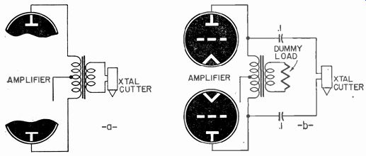
Fig. 1106--Two methods of connecting crystal cutter for constant-amplitude
recording.
Crystal Cutters
The crystal cutter, inherently a constant-amplitude device, can be made, however, to cut modified constant velocity very simply. With crystals, the turnover frequency can be varied at will merely by selection of the proper method of connection to the amplifier. Constant-amplitude records may, of course, be cut, too.
The crystal is a primarily capacitive device, and its capacitance remains, for all practical purposes, fairly constant at usual room temperatures. It has a definite (and different) impedance at different frequencies just as has a condenser. If the impedance of the crystal always exceeds, even at the highest frequencies, the impedance of the source of power which drives it, then the voltage across the cutter will be constant for all frequencies, and the cut will be constant amplitude. As an example the following specific data refers to the Brush RC-20 crystal cutter.
The RC-20 has a capacitance of .007 if. From the capacitive reactance formula : X, = it is seen that the impedance is approximately 225,000 ohms at 100 cycles, and about 2,500 ohms at 9,000 cycles. To cut constant amplitude, the driving source (output trans former secondary or tube plates) should have an impedance about that of the cutter at the highest desired frequency. If, with the RC-20, the highest frequency desired is 9,000 cycles, the source impedance should be 2,500 ohms although 4,000 ohms is adequate with this particular cutter. Two methods of connection for constant-amplitude recording are shown in Fig. 1106. The transformer--secondary (a) or the plate-to-plate (b) impedance should be equal to or less than X, at the top frequency. The maximum signal voltage across the cutter is specified by the manufacturer of each crystal cutter. For the RC-20 operating under these conditions, it is about 50 volts. Use a vacuum-tube voltmeter to measure this.
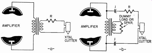
Fig. 1107--Crystal cutter connections for modified constant-velocity
recording.
If, when using the crystal cutter, the impedance of the driving source is made equal to the impedance of the cutter at any frequency, the cutter response drops at the rate of 6 db per octave above that frequency. The impedance of the .007 pi capacitance of the RC-20 cutter for instance, is approximately 44,000 ohms at 500 cycles. If it is fed by a 44,000-ohm source, response (stylus movement) will be constant for all frequencies below the 500-cycle point of equal impedances ; but, as the frequency rises, it will be reduced at the rate of 6 db per octave.
Under these conditions, the response is exactly the same as a magnetic cutter cutting modified constant velocity! Merely by adjusting the source impedance we can adjust the characteristic for any desired turn over frequency or we can cut constant amplitude, which is merely a characteristic in which the turnover frequency is above the usable frequency range, and so, practically speaking, does not exist.
In Fig. 1107, 2 methods are shown for connecting the crystal cutter to obtain the modified-constant-velocity response. In (a), the trans former-secondary impedance and the resistance of R each should be equal to 1/2 the impedance of the cutter at turnover frequency. In (b), the plate-to-plate impedance should be low (triodes or feedback-stabilized beam tubes should always be used and these will have a low plate-load impedance). R should equal cutter impedance at turnover.
In Fig. 1106-b or 1107-b the transformer-secondary load resistor may be replaced with a loudspeaker for monitoring, provided no equalization exists in the amplifier. However, the speaker alters the plate-load impedance with varying frequencies and so should not be used at the same time cutting is in progress. An ideal use for the speaker for play back of finished records is made possible by a simple switching arrangement.
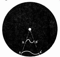
Fig. 1108--One cycle will occupy a much longer path on the disc at A
–A1, than at B-B1, with its more acute bends.
Refer to Fig. 1109.
In Fig. 1106-b or 1107-b the blocking condensers have a very high voltage rating, to prevent d.c. leakage to the cutter.
When modified-constant-velocity response is cut with a crystal cutter, driving voltage may be increased. With the RC-20, a turnover of 500 cycles will permit driving voltage of 150. Voltage overloads must be carefully avoided, or the crystal may be cracked.
After the crystal cutter is connected and the turnover frequency checked by observing the light pattern on a test record, the system is treated as though a magnetic cutter were used. Most crystal cutters do not have a flat frequency response. Excessive drop-off on either end, or a serious peak, may be corrected by equalization. The procedure is exactly the same as previously described for magnetic cutters.
High-Frequency Pre–Emphasis
After a good standard modified-constant-velocity response has been obtained, some thought can be given to special curves. Commercial phonograph records are made of a shellac compound, an abrasive included in it causing surface noise or scratch. Many phonograph users turn down the tone control to eliminate this, but, in so doing, they eliminate much of the high-frequency range of the record as well. For this reason, record manufacturers boost the high end of the range in recording. When this is done, using a tone control to reduce high-frequency surface noise brings down the boosted highs to the proper value. While this is not necessary with instantaneous discs because of their very low noise level, the recordist may want to try high boost on the premise that many cheap phonographs lack good high-frequency response. Experimentation is fairly simple, if the equalizer in the amplifier is sufficiently versatile. One record manufacturer, for instance, raises the high frequencies at the rate of 2 1/2 db per octave, beginning at turnover. This results in a 10-db boost at 8,000 cycles after which he cuts off the response very sharply.
Many phonographs are excessively boomy, so experiments with a bass attenuator may he fruitful.
In cutting discs at 33 1/3 r.p.m. we encounter an additional problem in equalization. Any cutting system which is properly equalized for 78-r.p.m. recordings, according to the outline given in this Section, will cut at the slower speed just as successfully when cutting near the outside of a 16-inch disc. When the diameter of the groove nears 12 inches, however, further treatment is necessary.
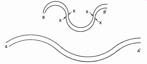
Fig. 1109--Grooves of same frequency at different disc diameters; note
pinching of groove at points X-X.
Fig. 1108 is a schematic drawing of a disc surface. When the disc revolves under the cutting stylus at a constant speed of 33 1/3 r.p.m., the stylus will take the same amount of time to travel from A to A', if it is near the outer edge of the disc, or from B to B', if it is near the center, since each of these distances represent the same fraction of a revolution. However, the actual linear distance travelled at BB'--with the cutter near the disc center--is much smaller than that traveled from A to A', when the stylus is near the edge.
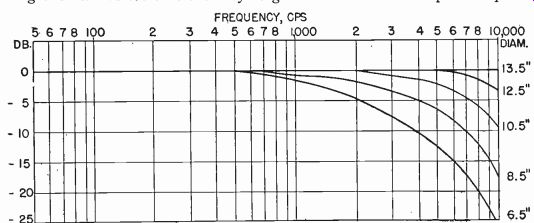
Fig. 1110--Approximate attenuation in payback due to "pinch effect" at
various diameters.
The drawing is much out of scale, but assume that the stylus travels each of these distances in 1/5,000 second. If the tone being recorded is 5,000 cycles the stylus will trace out 1 cycle in each case, as the drawing shows. Notice that the 1-cycle groove at AA' takes up a comparatively long distance and its undulations are fairly gradual. But at BB' the same cycle will have to be traced in a much shorter distance and its undulations are much sharper and its bends more acute.
Fig. 1109 is an enlarged view of each of these grooves. Notice that in AA' the width of the groove is fairly constant at all points. A reproducing needle of the proper size and shape will fit nicely into this groove and reproduce its variations faithfully. But in BB' the steeper bends of the engraved wave cause the groove width at points X to be perceptibly narrower than normal. Because of this, the playback needle will be forced up out of the groove somewhat; it will not track properly, and the output volume of the pickup will be decreased.
This pinch effect will occur to some extent no matter what the frequency. But, because the higher the frequency and the slower the disc r.p.m., the more the number of cycles engraved in a given distance, the effect is noticeable at 33 1/3 r.p.m. and at higher frequencies. In practice, pinch effect is not bothersome at frequencies much below 1,000 cycles, but if the playback needle is a little larger than optimum at its point, it will attenuate frequencies even lower than this. While the actual attenuation due to pinch effect in playback varies with the particular pickup and needle used, the curves in Fig. 1110 are typical.
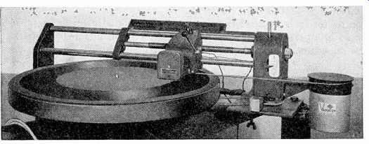
Fig. 1111-One type of automatic diameter equalizer mounted on overhead
lathe. The cutter pulls the string which regulates the equalizer setting.
Under a diameter of about 8 inches, the pinch is so great that little correction is possible ; but from 8 to about 13 inches, where the effect begins to be noticeable, diameter equalizers are used to correct the response. These high-boost (or low-pass) equalizers have 2 functions.
First, they boost the amplitude of high frequencies fed to the cutter (or attenuate the lows), the boost (or attenuation) increasing as the stylus travels inward on the disc. Second, they maintain over-all cutter level constant.
A number of amateur and semiprofessional recordists and all professionals use automatic diameter equalizers in which a variable control is geared to the cutter mount, so that as the cutter moves inward, equalization is automatically increased. Fig. 1111 shows one automatic equalizer, mounted on a recording assembly. A cord attached to the cutter mount turns the control within the cylindrical case. This unit, priced in the neighborhood of $75, is designed for insertion into a low-level, 500- ohm line, such as that between the console and the recording amplifier in the unit of Fig. 904, Section 9. Another type, priced considerably higher, is shown in Fig. 1112. The long flat box is mounted on the mechanism, parallel to the feed screw. A metal arm projecting from one of the long sides is attached to the cutter mount. The arm, moving with the cutter, contacts metal studs within the flat case. The studs are wired to the other box, which contains the actual equalizer. This unit is also designed for insertion in a low-level, 500-ohm line.
Diameter equalization can also be performed by hand. First, a high-boost or low-pass equalizer with a variable control is built into the system. Then a number of large discs are cut (without equalization) at various diameters with different frequencies. The playback response at each diameter and at each frequency is charted and compared with the response of a good 78-r.p.m. disc. A graph similar to that of Fig. 1110 is then made, and the exact position of the equalizer control for each diameter is determined. Usually adjustment every inch or so is satisfactory. The cutter level must be maintained constant at the same time. Doing this job manually is not only inexact, but it does not allow the recordist the freedom necessary to attend to other things.
An automatic equalizer can be made by ingenious constructors after a little thought and several tests.
Fig. 1112--Another automatic diameter equalizer. The flat box is installed
on the lathe.
Practical Equalizer Circuits
In the commercial line, a very popular low- and high-frequency-type equalizer is the resonant type allowing independent boost of highs and lows, with adjustable resonant frequencies. These are quite expensive but very suitable for high-quality professional installations.
Some types give attenuation at both ends of the range. Typical of these are the UTC 3A and 3D.
Thordarson offers a dual tone control of the nonresonant variety.
The kit consists of 2 special dual potentiometers and an a.f. choke. The circuit permits either boost or attenuation of both ends of the range independently. The actual Thordarson circuit may be found in the Thordarson Amplifier Manual, but it is actually an adaptation of a very useful idea--using degeneration for equalization.
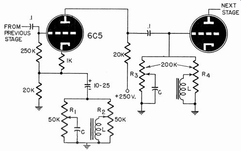
Fig. 1113--Circuit for universal equalizer.
Fig. 1113 shows a similar and very effective circuit which can be built without special parts. The 6C5 equalizer tube gives no gain unless either end of the range is boosted. It is to be inserted in an amplifier somewhere after the preamplifier stages.
When the arm of R1 rises, highs are boosted; when it is lowered to ground, highs become normal. When the arm of R2 is raised toward the cathode, the lows are boosted; when it is grounded, lows are normal.
When the arm of R3 is grounded, highs are normal; when it is raised, highs are attenuated. R4 controls attenuation of lows in the same manner.
Values of the condensers C and chokes L are not given because they should be determined by experiment and will depend on just what equalization is needed. The values will determine which portions of the range are affected. For example, with very small condensers, only the highest parts of the spectrum will be raised or lowered. If quite large values are used, the high controls will affect frequencies as low as 500 cycles.
The amount of boost or attenuation is controlled only by the potentiometers. L and C determine the frequency range affected. In practice careful measurements of the results must be made. Do not confuse the functions of the components. This excellent, all-around equalizer is to be inserted into the amplifier while it is being built, since, no matter what correction is later found necessary when cutting tests have been made, it is almost always possible to adjust the values of C and L and the settings of the controls for just the right effect. This unit will not take care of peaks in the range except at either end.
Resonant equalizers are most useful where very sharp boost or attenuation is required around a certain frequency. Usually the simpler nonresonant circuit will satisfy the needs of most recordists ; but where sharper curves are wanted, circuits similar to that of Fig. 1114 may be used. L and C are resonant at the desired frequency, and R1 adjusts the amount of equalization. R2 compensates for the change in level which occurs when equalization is varied. Two L-C combinations may be connected in series for equalization at 2 different frequencies.
It is seldom advisable to use resonant equalizers to compensate for peaks in cutter response. The peaks encountered in most units are not so sharp as to warrant elaborate L-C filters, and, when they are used for this purpose, an undesirable hangover effect makes all tones of the resonant frequency appear to linger for a period and die away gradually.
This effect is present whenever the cutter has a peak, but, while the equalizer may flatten the peak according to tests using an a.f. oscillator and an output meter, the hangover will still appear. It may even be accentuated.
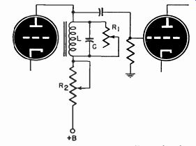
Fig. 1114--A resonant equalizer circuit.
Equalizers for use across low-impedance lines are hard to make because they must have a fairly good Q if they are of the resonant type.
Such units can be bought, however, from transformer manufacturers.
If control of frequency response is desired in a low-impedance line, the least expensive solution giving the most versatility in use is a small gainless amplifier inserted in the line. Any of the various high-impedance equalizer circuits which are presented in technical magazines, or the excellent one described here, may be used in this amplifier.
Reference to magazines and other literature is, in any case, a good way to discover many special-purpose equalizer circuits for particular requirements. While only one complete equalizer has been described in this Section, it is by no means the only suitable one. Equalizers especially designed for record playback will be found in Section 13. See also the GERNSBACK LIBRARY guide, AMPLIFIER BUILDER'S GUIDE.