THIS section will only discuss feedback as applied to power output circuits; other sections will deal with feedback where it is used for changing the characteristics of input circuits, for use as a cathode follower in the output of a preamplifier and for equalization circuits. However, we summarize here the basic theory of feedback in relation to its use for output circuits. Since much of this will apply to other circuits, it will not be repeated only the additional theory necessary for the particular application will be given.
Loop gain and feedback factor
In keeping with the purpose of this guide, we shall not give a detailed or rigorous presentation of feedback theory, merely a summary which will permit assessing the relative advantages and disadvantages of different feedback circuits. Taking the basic feed back amplifier (Fig. 301) we have an amplifying portion with a gain indicated by the symbol A. Some books, as well as articles, prefer to use the symbol µ to represent the gain of an amplifier. However, this author and the publishers prefer the symbol A to avoid confusion with µ as meaning the amplification factor of a tube. In dealing with feedback over only one stage, use of a symbol with two meanings would be particularly confusing because the gain of the stage is never equal to the amplification factor of the tube used in it. For this reason the symbol A is consistently employed to mean the gain, either of a single stage or of a whole amplifier.
The amplifier will have an output A times the input. For example if the input (eg) is 0.1 volt and A has a value of 180, the output (e0) will be 18 volts. As well as feeding whatever apparatus the amplifier has to power, this output is also returned through a feedback network. The voltage fed back to the input through the feedback network depends upon the feedback fraction {3. In the example we have chosen, assume that 1/20 of the output voltage is fed back; that is, 1/20 of 18 volts or 0.9 volt. The fraction f3 is 1/20 or 0.05.
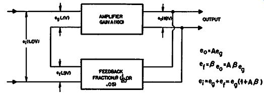
Fig. 301. Block diagram of amplifier employing overall feedback, showing
relevant quantities and formulas, and effect on overall gain.
We have, then, a "loop gain," as it is termed, through the amplifier and back through the feedback network of A Beta, or, in the example chosen, 180 X .05 = 9. This agrees with the fact that the 0.1 volt-input gives a fed-back signal (er) of 0.9 volt.
This must be negative feedback, to avoid producing oscillation, so the 0.9 volt must be out of phase with the original 0.1-volt in put. For a signal of 0.1 volt at the amplifier input, there is a fed back voltage of 0.9 volt so the preamplifier feeding it must supply, to overcome the 0.9-volt negative feedback, a total of 1 volt (e1 ). In terms of the circuit parameters, the input required from the preamplifier must be (1 + A Beta) times the original input without feedback. Increasing the input by the factor (1 + A Beta) to get the same output is the same as reducing the gain of the amplifier by this factor. This figure is what is termed the "feedback factor." In the example we used, A was 180 and {3 was 1/20 or .05, so A Beta = 180 x .05 = 9 and 1 + A Beta = 1 + 9 = 10. The loop gain is 9 and the feedback factor is 10. To summarize: Loop gain is the gain of the amplifier without feedback (A) multiplied by the feedback fraction (/3). In Fig. 301 it is the gain that would measure putting an input in at e_g and measuring the output at e_t.
Feedback factor is the amount by which the gain of the amplifier is changed by adding feedback or closing the feedback circuit.
In Fig. 301 it is the relation between the input without feedback (eg) and that with feedback (e1) to get the same output e0.
In amplifiers with the usual amount of loop gain, the two quantities are similar-they differ by only 1 and in a large number this will not seem much-so sometimes the terms are confused.
These facts have been explained in detail to clarify the distinction between the expressions "loop gain" and "feedback factor." Sometimes the figures are given in numerical quantities, in which case A is multiplied by f3 to get the loop gain. Sometimes A may be given in db and /3 also in db. A gain of 180, in the example noted, could be referred to as 45-db gain. The feedback fraction of 20 to 1 is an attenuation of 26 db so the loop gain is ~5 - 26, or 19 db, which agrees with the factor of 9 to 1 found by simple multiplication.
The loop gain in this example would be 19 db and the feed back factor 10, which may also be referred to as 20-db feedback.
The only simple way to obtain the relationship between loop gain and feedback factor is to use the numbers, rather than the db figures, which can add to the possible confusion.
Negative and positive feedback
The examples quoted refer to negative feedback. It is also possible, to a limited extent, to use positive feedback. The limit is that the loop-gain product A/3 must be less than 1. There are other practical limitations as we shall see further on.
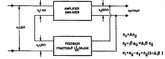
Fig. 302. Feedback can be positive as well as negative, increasing instead
of reducing gain.
Suppose the amplifier had a gain A of 20, or 26 db, and the feedback factor f3 is 1/25, or .04, which is 28 db; then the loop gain will be 20/25, or 0.8, which is -2 db (Fig. 302). If the amplifier input is 1 volt, the fed-back voltage will be 0.8 volt, in phase with the original 1 volt, the signal required from a preamplifier or external source need be only 0.2 volt. The gain now is modified by the factor ( 1 – A Beta) or 0.2.
In this example the loop gain is -2 db whereas the feedback factor is a positive one of 14 db, or a ratio of 5 to 1. The effect of feedback on the gain of an amplifier has been given first because all the other effects that feedback produces are in some way related to its effect on gain.
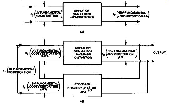
Fig. 303. Effect of negative feedback on harmonic distortion.
Effects on distortion
Assume that an amplifier has 4% distortion without feedback, a gain of 180 and an input of 0.1 volt. See Fig. 303. This means that, along with the 18 volts output, there will be a component -4% of 18 volts, or 0.72 volt-of distortion. This distortion may be harmonic, intermodulation or what-have-you, but it will be related to the signal. If the signal drops to 16 volts, the distortion will be 4% of 16, or 0.64 volt.
Look at the case with feedback. Theory tells us that feedback reduces distortion by the feedback factor-the same amount as it reduces gain. To verify this, fill in the figures and see how it works out. Our 20 db of feedback cuts the gain by 10: I-an input of 1 volt was needed, instead of 0.1 volt, to get the 18 volts output.
So the distortion should drop from 0.72 to .072 volt (or from 4% to 0.4%). The feedback will consist of a fraction of the distortion as well as the original signal, so we shall have a feedback voltage consisting of 0.9 volt of original signal and 0.0036 volt of distortion.
The 0.9-volt original signal is out of phase with the original 0.1 volt amplified, making an input of 1 volt necessary. But the 0.0036-volt distortion had no counterpart in the original signal so it will just be fed into the amplifier, along with the 0.1 volt, to be amplified. This will multiply it by 180, like any other signal the amplifier gets, giving 0.648 volt at the output. But this is in opposite phase to the original distortion component produced within the amplifier, which would have been 0.72 volt, so we are left with the difference of 0. 72 - 0.648 = .072 volt, which is the figure we assumed.
Weakness in theory
Although this is the usual way of stating the case with regard to distortion and feedback, there is something incompatible about it-for many purposes quite unimportant-but which does account for the discrepancy and, in fact, the breakdown in the application of this theory under some circumstances when we assume that the amplifier introduces distortion, this must mean that the gain of the amplifier changes during different parts of the waveform. An amplifier that maintains constant gain throughout the entire waveform being amplified cannot introduce distortion. This means that our use of a simple number, or algebraic system, to represent the gain of an amplifier is not strictly accurate.
In the example we assumed the gain to be 180. However, this must vary by at least 4%, from one part of the waveform to an other, if it is going to produce a distortion figure of 4%. A place where this principle interferes with the theory just developed is at the maximum output of a modern amplifier, usually limited by running into grid current clipping on the output stage.
When the output-stage grids start to conduct current, this is such a serious load on the previous stage that the voltage ceases to rise. Thus the signal at the grids is squared off at the voltage where the grid current starts and the voltage amplified beyond this point continues to be squared off. Hence there is a definite point at which the voltage excursion stops on the output waveform and, correspondingly, on the waveform passed back through the feed back.
Suppose that the input to this feedback amplifier is increased by 10% from the clipping point and that the clipping point occurs right at the 18-volt output (for simplicity we will assume that they are peak voltages rather than rms). When the input voltage reaches a value of 1 (and up to this point), feedback will reduce distortion and gain by the factor of 10 to 1 so at this point on the waveform there will be 0.1 volt across the input to the amplifier and 0.9 volt fed-back voltage to make up the combined input of 1 volt.
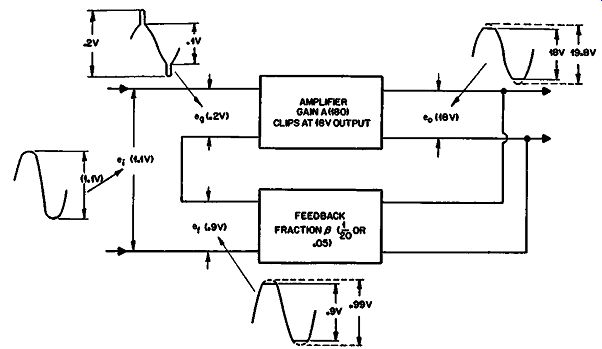
Fig. 304. Effect of feedback on distortion is strictly limited, particularly
when clipping occurs.
But now further amplification ceases: the fed-back waveform continues at the 0.9-volt level until the input waveform gets back to the 1-volt point at the end of the clipping period. So while the input waveform goes from 1 to 1.1 volts, the feedback stays at 0.9 volt and the amplifier gets the difference, which changes from 0.1 to 0.2 volt during this interval. An increase of 10% on the input waveform is accompanied by a peak that goes 100% higher at the amplifier input. The effect of this on the waveform is illustrated in Fig. 304.
Here we see a serious implication in the effects of negative feedback when an amplifier reaches its maximum output. For an increase of less than 1 db in the input signal, the level handled by the earlier stages of the amplifier rises by as much as 6 db. In the same amplifier an increase in input of 2 db, or 26% will step up the peak input voltage from 0.1 to 0.36, or more than 10 db higher.
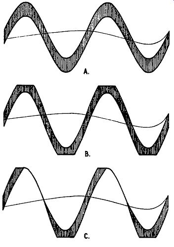
Fig. 305. Some effects of clipping demonstrated with the test waveform
used for IM testing. a--True composite; Waveform. b--Effect of clipping
in a well-designed amplifier. c--Waveform that occurs due to cyclic blocking.
Cyclic blocking
Provided the stages in the amplifier ahead of the final output can handle this increased level, there is no adverse effect except that the clipping is that much more sudden than it would be with a non-feedback amplifier. In other words, the feedback cleans up the waveform right up to the clipping point and then the clipping action occurs that much more suddenly because of the negative feedback.
But, if the earlier stages are not equipped to handle this sudden increase in level, further disadvantages can occur. Suppose that these sudden peaks cause grid current in one of the earlier stages which, due to the high circuit resistance there, alters the bias on this stage. when clipping has passed, the gain of the amplifier is liable to be changed-possibly even blocked, due to the change in bias.
This effect can be demonstrated with the aid of the kind of waveform used for IM testing, which consists of a 60-cycle wave with a 2,000-cycle wave superimposed on it. The waveform at the input is shown in Fig. 305-a.An amplifier operating without IM distortion will produce the same waveform at the output. When clipping commences under normal conditions, the waveform will be modified as shown in Fig. 305-b. But if the feedback signal causes some secondary blocking action, the waveform at the output is more like that shown in Fig. 305-c.
Avoiding overload blocking
·where an amplifier is poorly designed in this respect, a wave form of this type can occur when the input exceeds the maximum input permissible without distortion by as little as 1 or 2 db. How can this be overcome? In the average amplifier it is not feasible to make the first stage the one that overloads first with this increased peak signal from the feedback. Due to the small signals normally handled-in the region of 0.1 volt in the example quoted-there is bound to be a considerable margin, probably as much as 10 times, before serious distortion occurs in the first stage. The stage that is far more likely to run into distortion is the second stage of a three-or-more-stage amplifier.
This means that the second tube will be likely to run into grid current and produce erratic negative biases as soon as clipping occurs in the output stage. This is inevitable. The only thing that can be done is to arrange that it will not produce the kind of after effect shown in Fig. 305-c.
The simplest way to achieve this is to have the coupling between this and the first stage of the direct variety-in other words, no time constant due to the coupling capacitor. Then, although the second stage will still run into grid current which will drastically modify the waveform at this point, as soon as the grid current ceases the voltage on the grid will be back to its correct operating point instead of having become seriously negatively biased.
This feature of negative feedback amplifier design is an unsuspected recommendation for the long-tailed type of inverter.
Elimination of this particular coupling capacitor can also give advantages in attaining a satisfactory low-frequency stability margin.
Other effects of feedback Negative feedback also reduces spurious signals, such as hum and noise, by the same ratio that it reduces gain, provided these signals are generated inside the feedback loop. It cannot eliminate such signals that come in along with the input. This is not often of particular value in the output circuit. It can be of advantage when overall feedback is applied with a very-high-gain amplifier, but it is of more particular value in preamplifiers.
Stability of gain
Another important advantage of feedback is its effect not only on gain but on the stability of gain. Reverting to the example, in which the amplifier was assumed to have a gain of 180 without feedback: let us suppose that the gain falls by 10% due to a change in supply voltage or a defective component. This means that the gain will drop to 162, where previously it was 180. Using our formula, A has dropped from 180 to 162, but the feedback fraction f3 which we add has stayed the same-1/20, or .05. So the loop gain A/3 will drop from 9 to 8.1. Adding 1, the feedback factor, 1 + A/3 will drop from 10 to 9.1. This is the amount by which the input is reduced by feedback. Previously the 1 volt was divided by the feedback factor 10 to give 0.1 volt.
Now the same 1 volt will be divided by the feedback factor 9.1 to give 0.11 volt.
This will be multiplied by the changed value of A (162) to give the new output of 17.82 volts, which is a drop from 18 volts of only 0.18 volt, or a 1 % change in gain compared to 10% with out feedback.
So the use of feedback, giving an original feedback factor of 10, has reduced the effect of gain changes by this same factor of 10 (Fig. 306).
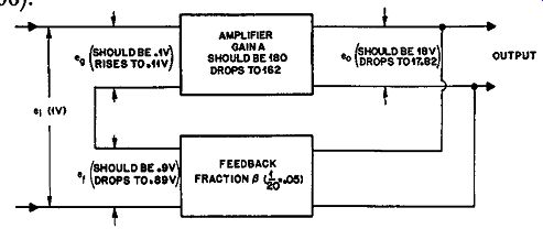
Fig. 306. Effect of negative feedback in stabilizing the gain of an
amplifier.
Frequency response
The general impression given by many treatments on the subject of negative feedback is that the feedback improves the frequency response in the same ratio as it affects gain. Sometimes this is deduced by quite involved theory and sometimes simply by a general statement from the material presented earlier.
The claim is that if the amplifier varies in gain due to change of frequency, the feedback will produce a corresponding reduction in the gain fluctuation as that described under the heading "stability of gain." The factor now introduced and which often gets overlooked is quite a fundamental one: any component which produces a variation in gain with frequency also introduces a considerable phase shift.
The foregoing discussion of the relation between loop gain and feedback assumes that the fed-back signal is either in exactly opposite phase to the input signal or exactly in phase. When frequency response comes into evidence, neither of these conditions is true, hence the magnitude and phase of the fed-back signal will not agree with either of the definitions given earlier for negative and positive feedback, respectively.
There is no simple and direct method of predicting the effects of a given amount of feedback on a specific frequency response.
The only way is to determine the exact frequency response of the amplifier with feedback in the following manner.
First, determine the frequency response, both in magnitude and phase shift throughout the loop (Fig. 307).
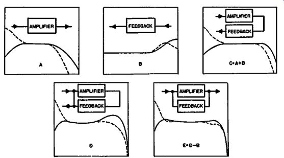
Fig. 307. The only, satisfactory way to work out the response of a feed
back amplifier: First work out the amplitude (solid line) and phase (dashed
line) response of the amplifier without feedback (A) and nf the feedback
(B), which combine to make the open-loop response (C). Then figure out
the effect of closing the loop (D). Finally subtract the response of
the feedback portion (E).
Second, from this information, the effect of closing the loop on the overall loop gain response can be predicted. This will, in general, depend upon how many stages of reactance elements contribute to the frequency response at each end of the spectrum and the relationship between the responses contributed by the individual elements. From this information, by appropriate calculation or the use of charts, the closed-loop response can be determined.
The final step is to subtract from the closed-loop response any response present in the feedback network. If some of the reactance elements contributing to the loop-gain frequency response are incorporated in the feedback network (contributing the function /3), then the response of the forward part of the amplifier with feedback applied will be the calculated frequency response of the closed loop minus the frequency response of the f3 section (Fig. 307). In considering the frequency response of an amplifier with feedback, a factor that must not be overlooked is the possible effect of the output load because this will invariably contribute one or more parameters to the overall open-loop response and hence also the closed-loop response.
Output impedance
Some think the use of feedback modifies the optimum load for a pair of output tubes. This basically is not true. The effect that feedback has on output impedance concerns the source impedance or resistance presented to the load and is used as a means of con trolling what is termed "damping factor." For triode type tubes the calculation of source resistance presented by a feedback amplifier is relatively easy, either by formula or by graphical method, using the tube characteristics (Fig. 308). First lay out the usual load line on the composite characteristics and calculate the swing voltages in all the circuit: plate volts 400 - 130 = 270; grid swing at output tubes 20; gain of amplifier "front end" 70; input to amplifier without feedback 20/70 = 0.286 volt. Fed-back signal is 1/420 of output or 270/420 = .643 volt. So the required input is 0.286 + 0.643 = 0.929 volt. This figure will be kept the same when the load is taken off. The off load condition is found by trial and error. When the plate swing is 300 at the output (400 - 100), the grid swing needs to be 15 volts. The amplifier input without feedback would then be 15/70 = 0.214 volt and the fed-back signal 300/420 = 0.715. Then the required input will be 0.214 + 0.715 = 0.929 volt, as before.
Larger and smaller swings can be tried until the right point is found.
We can now deduce the effective plate resistance. The plate swing changes by 30 volts (from 100 to 130 volts) for a change in current swing of 180 ma, representing a source resistance, referred to one half of the output transformer primary (see section 2) of 166 ohms.
If the feedback is of the current type, then it will be removed by taking off the load. On the other hand, removal of the load with voltage feedback will increase the resultant feedback. Either way, the result can be computed relatively easily from the curves or calculated from the following formulas:
Rn R. = ---- for voltage feedback;
1 +A/3 R. = Rn (1 + A/3) for current feedback.
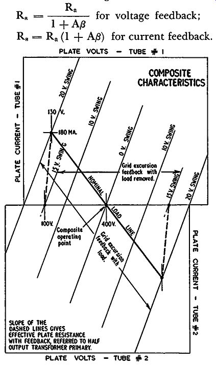
Fig. 308. Calculation of effective source (plate) resistance characteristics.
In each case R. is the source resistance and Rn the plate resistance.
The right values to use for A/3 are discussed later. This calculation is relatively simple for the triode tube because it has a fairly constant value for all its parameters. Throughout the operating range of all load lines, the amplification factor, plate resistance and transconductance do not vary very greatly in the whole region used.
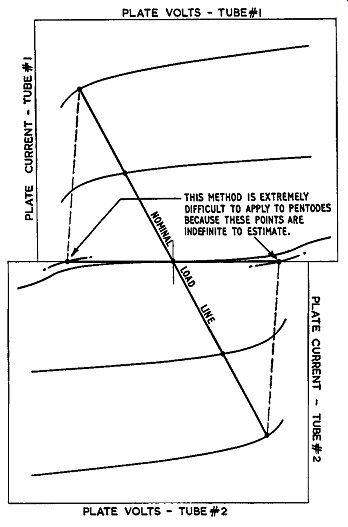
Fig. 309. Applying the method of Fig. 308 to pentode characteristics
is rendered difficult by the shallow slope and unevenness of curves.
But with pentode or tetrode tubes, the matter is not quite so simple. The amplification factor of output tubes is seldom given because it carries little meaning. The most constant parameter of this type of tube is its transconductance, but both the plate resistance and amplification factor vary widely at different points on their curves. For this reason it is impossible to estimate source resistance with a feedback amplifier from the parameters given numerically. It is not much simpler using the characteristics, as will become evident from Fig. 309--only an approximate estimate can be achieved at best. The method is similar to that used for the triode. The difficulty is that, on the open-circuit condition, in the case of voltage feedback, the composite curves are difficult to construct because the individual curves close up and have erratic curvature. Hence it is difficult to tell where the dot and dash lines of Fig. 309 should be, and what voltage they represent. Hence the exact voltage swing obtained on open circuit is very difficult to determine. The effect of current feedback is even more difficult to judge because of the difficulty in reading the quantities involved.
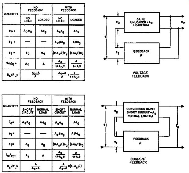
Fig. 310. Deduction of the effect of voltage and current feedback on
source resistance from first principles.
The general effect of feedback on source impedance can be deduced in a manner similar to that used for distortion and gain stabilization, from first principles, as shown in Fig. 310. The difficulty is that the source resistance in the absence of feedback must be known. While the triode readily provides such information, the pentode or tetrode yields a source resistance which varies widely throughout the operating cycle.
To illustrate, in a triode amplifier, suppose that without feed back, the output e drops from 10 volts without load to 4 volts with the load connected. If the input e1 is 1 volt, A, of Fig. 310 10-4 is 10, and A is 4, so R./Rr, = ---= 1.5. The source resistance 4 is 1.5 times the load resistance. Now suppose that, without the load, 4 volts, or 2/5 the output voltage, is fed back. f3 is 2/5. The input e1 will now need to be 4 + 1 = 5 to get 10 volts output. The feedback factor, without load (A0/3 + 1) is 4 + 1 = 5 so the source resistance with feedback should be 1.5 x 1/5 = 0.3. Put ting the load on should now drop the output voltage from 10 to 10/1.3 = 7.7. We can now check this. 2/5 of 7.7 volts is fed back, or 3.08 volts, leaving 1.92 volts of the original 5 at the amplifier input. The original gain with the load connected was 4, so the output will be 4 x 1.92 volts, which is as near to the figure of 7.7 as calculation will give because 10/1.3 is not exactly 7.7.
The application of a given amount of feedback measured, in the case of voltage feedback, without the load connected and, in the case of current feedback, with a short-circuit condition, will modify the natural (no-feedback) source resistance of the amplifier by the feedback factor.
The computation of effective source resistance must be made either open-circuit or short-circuit, according to whether voltage or current feedback is considered. If the gain and feedback characteristics of the amplifier are considered with the nominal load connected, the same theoretical result can be obtained, provided the following procedure is adopted.
First, the gain of the amplifier is calculated with the load connected, hence the feedback factor is based on this calculation.
The source resistance of the amplifier is also calculated with the load connected. This consists of the plate resistance of the output tubes in parallel with the load connected for voltage feedback, or in series for current feedback.
The output resistance is then divided or multiplied, according to whether voltage or current feedback is used, by the feedback factor. The resulting impedance is a combination of the source resistance of the amplifier in parallel or in series with the load connected.
Suppose that the optimum load for the output tubes is 6,000 ohms plate to plate and each has a plate resistance of 50,000 ohms, making 100,000 ohms plate to plate. Finally, with the load connected, the feedback factor is 10 (i.e., 1 + A/3). The combined resistance of 6,000 and 100,000 ohms in parallel is 5,660. Voltage feedback will reduce this to an effective parallel resistance of 5,660/10 or 566 ohms. As this consists of the actual load, 6,000 ohms, in parallel with the new value of source resistance, we can 566 X 6,000 deduce that the source resistance is --- = 625 ohms. In 6,000-566 other words, the source resistance (625 ohms) and the load resistance (6,000 ohms) in parallel make the calculated value of 566 ohms.
The choice of method will depend upon the circuit. In pentode circuits the open-circuit gain is difficult to calculate so this second method is better. For circuits where the plate resistance and open circuit gain are easy to calculate, the first method, using open circuit feedback factor, is simpler and less confusing.
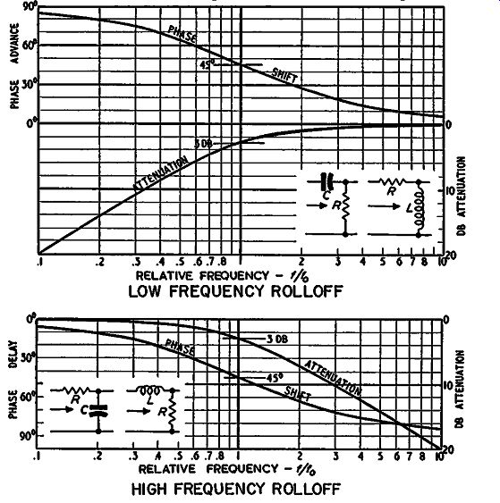
Fig. 311. Standard rolloff characteristics for a single reactance, contributing
to low- or high-frequency loss. Curves are plotted to a relative frequency
in which reactance is equal to circuit resistance R.
Stability margins
We have talked about negative and positive feedback as if they are definite entities that can be kept in convenient separate compartments. Unfortunately, they are not quite so in practice. What we design as negative feedback can become positive at some frequencies. In the formula for positive feedback, if A/3 is made equal to 1, the gain will jump to infinity, which means the amplifier will oscillate. Referring to Fig. 302, the signal fed back is equal to the original input-the amplifier supplies its own input and oscillates.
For negative feedback to become positive, become unstable, and start oscillation, it must undergo a change: its phase must reverse, or change through 180°, and there must still be at least as much signal fed back as the original input. In terms of the formula, A Beta must be 1 or greater.
Feedback does not suddenly change from negative to positive it goes through a gradual transition. The reactances that cause ultimate phase reversal cause a progressive phase advance or delay.
Reactances, such as coupling capacitors, that are responsible for low-frequency rolloff cause a phase advance. Reactances, such as stray capacitance and leakage inductance, that cause a high-frequency rolloff introduce a phase delay.
A single reactance causing a rolloff simultaneously produces a progressive phase advance or delay with changing frequency which reaches an ultimate of 90°. At one particular frequency on this rolloff an interesting relationship holds. This is where the attenuation or amplitude loss is 3 db and the phase shift is half of the ultimate, or 45°. (Fig. 311). If in a whole amplifier there are two reactances contributing to such a rolloff and they both act at the same frequency, the loss will be a total of 6 db and the phase shift 90°. Ultimately at extreme frequencies, when there is considerable attenuation, the phase shift approaches 180°. In theory it never reaches 180°, only approaches it more closely with increasing attenuation.
When we move on to three reactances contributing to a rolloff at the same end of the frequency response in an amplifier, if the three reactances produce identical rolloff characteristics-that is, the 45° and 3-db frequency points are identical-then the cumulative effect will produce 9 db loss and 135° phase shift. A little farther along, each rolloff will be giving 60° phase shift and 6-db attenuation. The cumulative effect of the three networks is 18-db attenuation and 180° phase shift.
Obviously in this case, if the loop gain also happens to be 18 db at the frequency in question, we have a positive feedback condition with 180° phase shift and a fed-back signal equal to the input signal-just enough to cause oscillation. This is the instability point for this particular network.
Negative feedback is designed to reduce the gain (and other things that happen with it) by a large factor, such as 10 to 1. The loop gain A_Beta is correspondingly large for most frequencies. But, when the circuit reactances start to take effect, two things happen: there is a progressively increasing phase shift and the gain A drops off. When the change of frequency brings the phase shift up to 180°, the feedback has completely changed from negative to positive. What happens here is determined by the value of A_Beta at this frequency. If it is more than 1, the amplifier will go into oscillation at this frequency. If it is less than 1, the amplifier will not oscillate but the feedback will boost gain at this frequency instead of reducing it.
We can state the condition for stability in two ways: (a) when the phase shift reaches 180°, the loop gain must be less than 1 and (b) when the loop gain falls to 1, with increasing (or reducing) frequency--and until it falls to 1 -- the phase shift must not reach 180°. Any amplifier with three or more reactances contributing to rolloff at the same end of the frequency response can reach an unstable condition if the loop gain is sufficient for the particular combination of rolloff parameters. If there is only one roll-off in the feedback loop it is impossible to produce instability, or even peaking, in the frequency response. If there are two rolloffs at the same end of the frequency response, instability can never occur, but it is possible to produce peaking.
The possibility of instability has long been recognized as an important design limitation because it makes itself noticeable so very definitely. An amplifier that goes into oscillation is unusable.
The design of feedback amplifiers has long included procedure for ensuring a margin of stability.
This can be specified in two ways to correspond with the two ways of expressing the condition for stability. These are called phase margin and gain margin. Both are related to the loop-gain characteristics, and particularly the way these change with frequency. One uses the frequency where the loop gain reaches 1 (as it drops off) as a reference, while the other uses the frequency where the phase reverses (reaches 180°). They can both be calculated, but phase margin is difficult, if not impossible, to measure.
Phase margin
At the frequency where the loop gain A_Beta has fallen to I-that is, the gain of the amplifier is only just equal to the feedback fraction, the phase shift must be something less than 180° to in sure stability. The amount by which the phase at this frequency comes short of 180° has been called the "phase margin." This is easy to define but not quite so easy to measure.
Gain margin
The better form of margin, from the viewpoint of measurement and checking, is the gain margin. This is the amount by which the loop gain A/3 is below 1 at the frequency where the phase shift is 180°. This can be checked by increasing the amount of feedback until instability occurs and then comparing the amount of feed back at which instability occurs with that actually used. (Fig. 312).
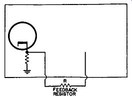
Fig. 312. Measure the gain margin by adjusting the feedback until the
amp oscillates.
If the difference is, say, 6 db, then this means there is a 6-db gain margin. Many books on amplifier design give recommended figures as to both phase and gain margin for satisfactory performance. But what this method of specification does not show is the peaking that can occur in the frequency response, even though the amplifier is quite stable.
Maximal flatness
To avoid peaking at any point in the frequency response, even beyond the audio band, a margin considerably in excess of 6 db is always required. This can be particularly seen in the kind of amplifier that has only two reactances contributing to high or low rolloff. However much feedback is used, this amplifier does not become unstable; but it can run into very high peaks at the extremities of the response.
When three or more reactances for each end of the frequency response are used in the feedback loop, there is a definite margin between the point where peaking commences due to the feedback and where the amplifier runs into instability. The point where peaking commences can be regarded as the point of maximal flatness. From the viewpoint of overall performance this is the best point at which to operate an amplifier.
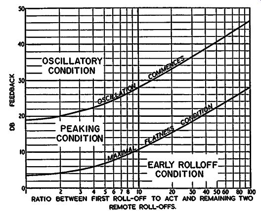
Fig. 313. Basic relationship for various operating conditions in an
amplifier with three reactances contributing to rolloff at one end of
the frequency response.
Figs. 313 to 315 show the margins necessary between the be ginning of peaking and the instability point for different combinations of rolloff point in the amplifier loop-gain characteristic, using three, four and five reactances contributing to the rolloff characteristic.
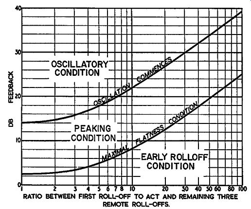
Fig. 314. Amplifiers using four reactances contributing to low or high-frequency
loss.
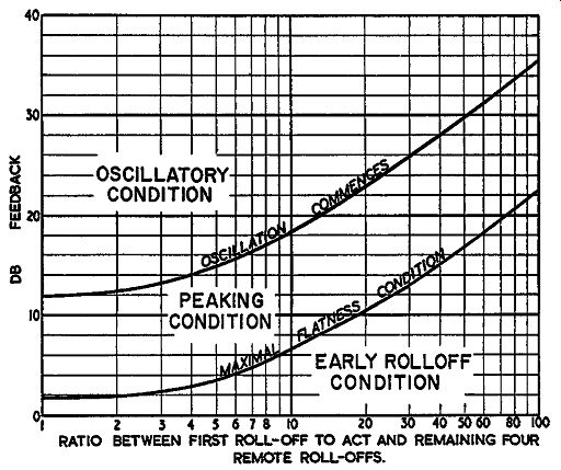
Fig. 315. Five reactances contributing to the rolloff characteristic.
Good design
The general philosophy in designing an amplifier according to this data is to have one of the rolloffs in the circuit nearer to the audio band than the rest. This allows for the maximum amount of feedback with the particular spread in rolloffs chosen.
Take the amplifier shown in Fig. 316, for example, in which the four reactances contributing to high-frequency rolloff are: (1) the plate-to-ground capacitance of the first stage (including grid-to-ground capacitance of the second stage), (2) capacitance between grids of the output tubes (with ground as a virtual center point), (3) plate-to-plate capacitance of the output tubes (including primary capacitance of transformer), (4) leakage inductance between primary and secondary of output transformer.
Fig. 314 shows that for four-stage cases 20 db of feedback requires a rolloff ratio of 55 to produce maximal flatness. A lower ratio will result in a response that peaks, while a larger one (very difficult and therefore unlikely to achieve) would result in a response that rolls off earlier and more gradually than the maximal flatness curve.
For maximal flatness, the rolloff (3) could be set at 20 kHz and (1), (2) and (4) at 1.1 mhz. This does not mean that each has to be exactly at this upper frequency, but rather that this frequency should be regarded as a minimum. This is a difficult design to achieve, especially getting the leakage inductance that small.
Fortunately, we do not need to stretch things quite this far, because the feedback will extend the overall frequency response considerably-in fact almost to the outer three rolloff points. A satisfactory design could be based on placing the upper three roll offs at between 80 and 100 kHz and then making the first one act at this frequency divided by 55-somewhere in the region from 1,500 to 1,800 Hz. This would mean that the loop gain A/3 would begin to drop below 20 db at frequencies above, say, 2 kHz so that the full 20-db feedback would not be available for reducing distortion above this frequency. However, the amplitude at frequencies above this never reaches maximum and so the full distortion-cancelling effect of feedback is unlikely to be necessary.
Certainly, it is never necessary to realize 20-db feedback at 20 kHz because any amount of distortion at 20 kHz is not audible-in fact 20 kHz itself is not audible to most ears! But, taking even the high est audible frequency, its second harmonic is definitely not audible so considerable distortion of this frequency can be permitted because the distortion components are also not audible. However, the fact that the components at this frequency are very small means that little distortion will occur to need cancelling.
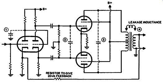
Fig. 316. Typical feedback amplifier.
At the low-frequency end the problem can be a little tougher.
A fair amount of power is required at least down to 100 Hz. It is not feasible to set most of the rolloffs down in the region of 1 or 2 Hz because of the oversize capacitors involved. A saving factor can be the use of direct coupling to reduce the number of reactances contributing to low frequency rolloff.
This may seem strange to many who have become used to the idea of a feedback amplifier that has a response extending way beyond 20 kHz and with very low distortion within the entire audio band. To confirm the validity of our theory, let us see some of the possible ill results of more conventional amplifier design.
Super-wide-band fallacies
Very little distortion shows up over the frequency range under test conditions. But what happens on square waves and other kinds of transients? Due to the fact that an amplifier so designed must inevitably possess peaking at some frequency beyond the audio band a ringing condition is set up within it. This means that, momentarily, signals of excessive amplitude at some frequency-probably in the region of 200 kHz to 1 me-will circulate around the feedback loop. This can happen although, in some amplifiers, no ringing shows up in the output. If a single test square wave is the source of this excitation, the family of frequencies set up will be interrelated and cannot produce any spurious components down in the audio band.
However, practical transients are not perfect square waves-the clash of a cymbal and various percussion sounds are not anything like the square-wave transient used for testing-and consequently contain a number of sharp exciting basic waveforms that set up a complicated pattern of frequencies in the region of the feed back peak. This means that IM distortion occurring round the feedback loop will introduce spurious components, some of which are within the audio band.
At the peaking frequency, the feedback has virtually disappeared as far as cancellation is concerned. It has, instead, turned into positive feedback and is almost reaching the point of oscillation. So these frequencies will be accentuated and the distortion characteristics of the amplifier, normally cut back by 20 db, are receiving full accentuated sway as far as these signals are concerned. These, then, generate IM among themselves, some components of which will be in the audio band and appear at considerable amplitude.
True, the feedback is operative at these frequencies and will reduce them by the 20-db feedback applied, but they can still be sufficient to be audible and to make reproduction harsh, gritty or muddy.
This ringing occurs even in some amplifiers that appear to give a satisfactory square-wave response. This can be demonstrated by measuring waveforms at various points (Fig. 317), which prove that the good wave at the output is obtained by skillful balance, or null adjustments, of the ringing. This does not prevent the effects just described, however.
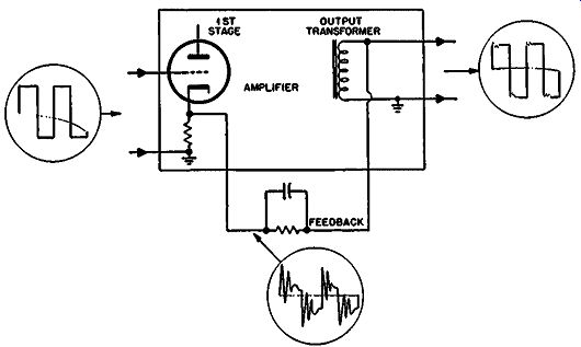
Fig. 317. Excessive ringing, skillfully balanced in the output.
The low end too
There is another kind of distortion that occurs regularly, due to subsonic peaking at the low end. Many feedback amplifiers may be quite stable at low frequency but, as in the case of the high-frequency response, the stability margin is probably in the region of 6 db. This means that there can be a very consider able peak at a low frequency-probably 1 or 2 Hz. This enables the amplifier to give an extraordinarily good frequency response as measured by conventional methods. It will probably be within 0.1 db, down to 20 Hz. This does not mean however, that it may not have a IO-db peak at about 1 cycle.
And how does this cause distortion? If the low-frequency peaking is increased to the point where it just causes instability, the amplifier will go into full amplitude oscillation at 1 or 2 Hz.
Even on many good speakers this will not be audible because the frequency is too low to move the diaphragm at appreciable amplitude. Probably also the output transformer has low-enough inductance so that there is insufficient coupling from the output stage to drive the voice coil appreciably at this frequency.
However the oscillation will be very evident inside the amplifier itself. The B-plus line will be fluctuating violently and all of the tube operating points will be amplifying a large amplitude signal.
This means that the gain of every stage throughout the amplifier will be fluctuating quite widely due to this large amplitude signal passing through. In turn this will cause an unusual kind of inter modulation distortion of any program material that happens to be amplified at the time.
This is one explanation of why amplifiers that give a very low measured IM distortion sometimes produce quite audible IM distortion under practical program amplification, even at low levels where distortion caused by clipping does not occur.
To complete the picture we need to know the answer to the question, "What kind of transient will start this?" Any kind that produces a "temporary de" component in the waveform; that is, a kind of program waveform that is asymmetrical. ·with an old type amplifier without feedback this means that all the bias operating points will need to readjust themselves due to the asymmetry. However, in a feedback amplifier, when there is instability or peaking at this low frequency, the progressive readjustment through the amplifier will become exaggerated and sets up a low frequency oscillation (Fig. 318).
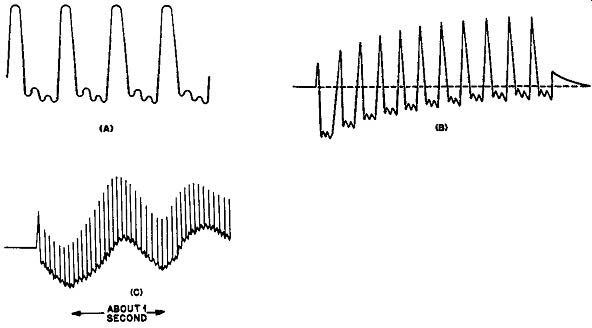
Fig. 318. Effects that can occur with an asymmetrical waveform: a-typical
wave form; b-how a single R-C coupling re adjusts to this waveform; c-when
a complete feedback amplifier bordering on low-frequency instability
handles it, a spurious low-frequency fluctuation is induced.
Typical program material that can initiate this are the plucked string instruments-particularly string bass, the drums and also many of the wind instruments, such as the trumpet. These last produce an asymmetrical waveform when viewed on the scope, probably due to the fact that there is a "de" component caused by the wind blown through the instruments. Whatever the cause of the asymmetry, its effects can be very drastic in this kind of amplifier and cause considerable distortion even though the amplifier's specification shows it to be indistinguishable from perfect.
Loading
There is one more feature to watch in this matter of stability criteria, or margins, in amplifiers. Test conditions specify that the amplifier has a resistance load. According to specification, this means that, when the output impedance is specified at 16 ohms, the performance of the amplifier is measured with a resistance load of 16 ohms connected to it.
However, we do not listen to resistance loads; we listen to speakers and they do not have a pure resistance as an impedance.
They may have an impedance of 16 ohms at one frequency, probably in the region of 600 Hz, but at other frequencies the impedance deviates quite widely. Down at a low frequency, in the region of the speaker's natural resonance, the impedance may well be as high as 50 ohms and in this region it will possess quite considerable components of reactance. Also at the high-frequency end there will be substantial reactance and the impedance will tend to rise.
When speakers use crossover networks, the matter is further complicated by possible reactances introduced by the crossover arrangement. All in all, the load looks very much different at all points from a true resistance load as specified for many of the amplifier tests.
Some thank that if you design the amplifier with a good high damping factor, this will not matter-the feedback takes care of the amplifier and it doesn't matter what load is connected. Un fortunately, this is not necessarily true.
Assume the amplifier uses a pentode output stage in which the normal load impedance is about one-tenth of the source resistance presented by the output tubes. Using the simplified method of calculating with the load connected, a source resistance of one tenth of the load resistance (or a damping factor of 10) can be achieved by using about 20-db feedback when working into the correct resistance load. This arrangement may perform perfectly but notice what happens as soon as the load changes, due to the fact that the output stage source resistance is actually 10 times that of the load resistance.
Without feedback, the voltage would rise by approximately 10 times when the load is removed. However, applying the same feedback circuit will knock the output down to the same figure it did when the load was there -- within 10%. This means that the feedback has risen from its nominal value of 20 db to something probably in excess of 40 db.
If the stability criteria were calculated or measured on the basis of 20-db feedback using the correct nominal load, something very different can happen when the load is removed, allowing the feed back to rise to 40 db, and when intermediate conditions of loading are used with reactance. The amplifier has a great variety of possibilities in achieving a satisfactory stability margin. Obviously there are big--if not impossible--problems in designing such an amplifier successfully so that it will always perform equally well.
Multiple-loop feedback
The solution rests in the employment of multiple loops. Re member that feedback over only one reactance cannot cause peaking under any circumstances. So then, the best method is to apply feedback directly from the plate circuit of such an output tube to the grid or drive circuit of the same tube, to reduce the source resistance to something comparable with the nominal load resistance. This will be about 20 db of feedback. Then, having stabilized the source resistance and gain of the output stage to some extent, further feedback can be used on the overall loop to achieve a satisfactory damping factor without running into such severe complications (Fig. 319).
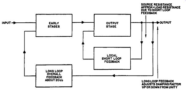
Fig. 319. Choosing the best balance between short and long-loop feedback.
It is appropriate here to insert a note on the relative advantages from the feedback viewpoint of different types of operation of output tubes. Triode operation yields a low source resistance, hence does not require local-loop feedback to stabilize the source resistance before applying a long-loop feedback. Ultra-linear, in effect, has a local-loop feedback in the form of connection to the screens and so achieves an objective similar to the triode. Pentode operation, however, should still use some local feedback to re duce the effective source resistance into the region of the load resistance before applying an overall feedback loop.
Phase correction methods
A common method of amplifier design consists of what might be termed "cooking" the stability margin by placing small values of capacitance in various places in the amplifier circuit. This produces what are virtually step or shelf responses in the overall loop gain. A popular position for such a "cooking" capacitor-normally given the better-sounding title of "phase-correction" capacitor is across the feedback resistor itself (Fig. 320).
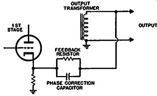
Fig. 320. Use of so-called phase correction capacitor in feedback
amplifier design.
The whole amplifier is carefully adjusted by means of this and other small capacitors so that the frequency response meets the specification throughout the required frequency band and so that there is what is considered to be a satisfactory stability margin in the order of 6 db.
The obvious way to see the defects of this method is to consider this design as a feedback tone-control circuit. The capacitor in parallel with the feedback resistor means that the feedback net work gives a "boost" to the high frequencies. This should, in con junction with a "perfect" amplifier, produce a rolloff in the high frequencies in the overall response of the amplifier measured from input to output. However, the amplifier has been "juggled" so that the overall response is perfectly flat. If there is a boost in the feedback section, this means that the overall loop gain, measured from input of the amplifier back to the return point from the feedback, has a high-frequency boost in it. Although the overall response, measured from input to output, may show perfectly flat, the loop-gain response inevitably has a peak because of the way in which the response is achieved.
This author has conducted some tests on amplifiers designed along these lines and revised the circuitry to fall in line with sound practice. The rolloff characteristics were adjusted to give a sufficient stability margin to insure no peaking. As a result the response of the amplifier, it is true, no longer stayed within the fine tolerances stated in the specification-which were in the region of 0.1 to 0.5 db from 20 Hz to 20 kHz for different amplifiers.
However, the response was still what can be considered acceptable for true high quality-within a loss of 3 db at each end of the audio-frequency response. This certainly cannot be detected audibly and, by doing it in the correct way, the amplifier sounds considerably cleaner on all kinds of program material than with the arrangement artificially extended within fine tolerances.
Multiple-loop interaction
There are some further aspects that should be considered in a little more detail (Fig. 321 ). Here we are considering the local loop current feedback at the input stage in conjunction with the overall loop feedback from the output stage.
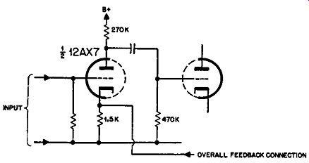
Fig. 321. Interaction between feedback in two loops.
Before a connection is made for the overall feedback, there is local current feedback on the input stage itself. Using the values shown, the half of a 12AX7 tube gives a gain of 67. The bias resistor of 1,500 ohms in conjunction with an effective plate load of 270,000 ohms gives a fractional feedback of 1/81. So the loop gain is 67 /81 or 0.83 and the feedback factor is 1.83. This represents a feedback of 5.25 db. Assume that the amplifier is designed on the basis of 20-db overall feedback. The loop gain from input to output and back through the feedback should be 9. Now 1 volt in from grid to cathode of the first stage will produce 0.83 volt due to local feedback and 9 volts due to overall feedback. The overall reduction in gain is a ratio of 1 to 10.83, or 20.7 db. Now we see that the overall feedback is giving us 20 db whereas the local feed back has reduced from 5.25 to 0.7 db, due to the connection of the overall loop.
A similar variation happens between the loops of Fig. 319.
Without a load connected, the local loop gives 20-db feedback and the overall loop 20 db more, with the correct load connected, the local loop drops to about 5 db and the overall loop to about 15 db.
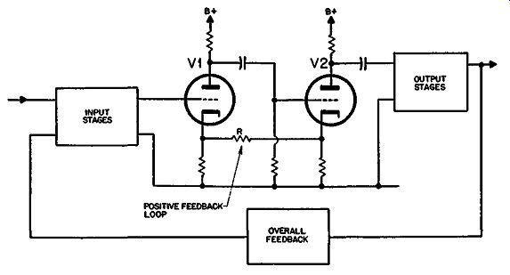
Fig. 322. Another case illustrating interaction between feedback
loops.
"Infinite-gain" stage
The infinite gain stage is another example (Fig. 322). Infinite gain is achieved by connecting the resistor R between cathodes of the two stages shown. This means that the signal at the cathode of the first tube is equal but in opposite phase to the signal at its grid. This anti-phase voltage is derived by feedback from the cathode of the second tube shown, which cancels the current fluctuation due to the first tube itself and exceeds it to this extent.
If the grid of the first stag-e is considered as strapped to ground, this two-stage setup will oscillate freely at a frequency determined by the reactances of the overall arrangement. This will cause phase shift to prevent oscillation at frequencies other than the center of the band. If feedback in excess of a loop gain of 1 is employed, the oscillation will become "harder," producing a squared or clipped waveform, until the effective loop gain averaged over this distorted waveform is 1.
Assume the overall loop applies what would be 20 db if the positive feedback were not present-that is, if R were removed. As a start, assume a signal at the plate of the first stage shown that would normally be occasioned by 1 volt from grid to cathode. Due to the 20-db negative feedback there will be 9 volts in opposite phase delivered via the output, feedback loop and input-that's assuming nothing runs into distortion. This would be so wherever you start the consideration of a feedback amplifier. It can be shown at the input because 9 times the input comes back in opposite phase from the feedback network, but when the input circuit is closed, the same thing will happen if the amplifier loop is opened at any other point.
When R is connected, there is an equal voltage of 1 returned from the cathode of V2 so that the two stages would go into oscillation. But at the same time, due to the same hypothetical initiating voltage of 1 volt between grid and cathode of V1, the overall negative feedback loop will return an anti-phase voltage of 9 volts to the grid. So now the overall effect with the positive loop feedback between cathodes is as if the negative feedback loop had a loop gain of 8 instead of 9. In other words, the effect of closing both loops now has a net change on this stage of 19 db.
However, the overall feedback has been set at 20 db, compared to the condition without positive feedback. The fact that there is now only an apparent negative feedback (referring to this stage) of 19 db, indicates that the positive feedback, instead of being in finite as in the absence of the negative feedback loop, now merely boosts the gain of this stage by 1 db-the difference between 19 and 20. It's all a question of viewpoint. ·when you consider the overall amplifier, there is still an apparent gain of infinity before the negative feedback loop is connected. So it is possible for some things to be done, using this circuit arrangement, that are not possible with a simple straightforward 20-db negative feedback.
But we have to be careful how we apply this thinking.
If the infinite-gain stage produces any distortion, this is likely to get magnified. Without the negative loop feedback from output to input, the stage has infinite gain and considerable distortion (self-generated). Applying the negative loop feedback brings the gain down from infinity to some finite value and at the same time restricts the distortion in this stage-or would do so if the negative feedback had no distortion elements of its own. But, because of the distortion elements in the negative loop feedback, particularly the output stage, this fact is no longer true and the distortion elements themselves will interact in a way that becomes somewhat complicated to predict.
This can be particularly troublesome when the output stages are driven to clipping point. Then the negative feedback momentarily disappears, leaving the "infinite-gain" stage free to "take off" until clipping ceases.
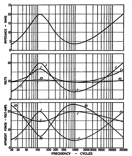
Fig. 323. Impedance characteristic of a speaker affects the response
fed to it, using different damping factors.
Positive feedback has some limitations associated with overall stability and response criteria. Over a single stage, feedback merely modifies bandwidth-positive narrows it, negative widens it-and the overall criteria are simple resultants of both forms. If positive feedback is used over more than one stage, the bandwidth is still narrowed but the associated phase shift is no longer simple so the ultimate interaction with a negative feedback loop can produce complicated and almost unpredictable results.
Variable damping
Variable damping in itself produces some fundamental problems. If the speaker were a pure resistance, the question of damping would be quite unnecessary because a resistance is critically damped in itself. However, since a speaker possesses both electrical and mechanical or acoustical forms of reactance, damping is necessary. Unfortunately, the fact that these reactances are present causes the speaker to have a somewhat complicated load-impedance characteristic. This means that the frequency response of the energy fed to such a load will vary according to the resistance source from which it is fed.
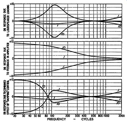
Fig. 324. Performance of a variable damping control that uses current
feedback at the low-frequency end only, Top-variation in frequency response
caused by different damping factors acting with the speaker impedance
characteristic ( as in Fig. J2'J ). Center-amplifier response changes
as the damping factor is changed. Bottom-combined response due to both
effects acting together.
If the source resistance is zero, the voltage across the load will be constant at all frequencies. As soon as the source resistance is increased fo some finite value, the voltage across the load will follow the general contour of the impedance characteristic (Fig. 323). Variable damping aims to eliminate undesirable resonant effects from the speaker by damping transient vibrations. This is not directly connected with the frequency response of the instrument and should be considered as a completely separate form of distortion. However, as soon as you start to adjust the resistance from which the loudspeaker is fed, you will also alter the frequency characteristic it gives.
Some of the earlier damping-factor control circuits compensated for this by arranging that the adjustment in feedback occurred only at low frequencies. This is where control of damping is most desired. By varying only the current feedback at low frequencies and keeping the component of voltage-feedback constant, the gain of the amplifier at the low-frequency end was modified by the damping factor in a manner approximately inverse to the effect of this control on the frequency response due to the impedance characteristic of the loudspeaker (Fig. 324). Unfortunately however, in designing the amplifier, the compensation has to be judged for the average speaker; that is, the change in current feedback takes over at a specific frequency de signed into the amplifier. This may or may not agree with the position of the change in impedance of individual speakers.
Although this compensation does to some extent level off the response variation above the resonant frequency in the electrical impedance characteristic of the speaker, the variation is exaggerated at frequencies below this point. This means that going into the region of positive current feedback-which is the maximum or negative damping-factor region-the response is exaggerated at points below speaker resonance. This will include rumble frequencies and similar components from the amplification system, hence results in an undesirable exaggeration of any subsonic frequencies present. If, in addition, the amplifier has a peak in its low-frequency characteristic due to poor stability margin, the distortion introduced can become considerable although this might appear to be the optimum damping for a particular speaker.
At best, any attempt to control the damping factor must be a compromise. It seems that the change in frequency response, due to the impedance characteristic of the speaker, which inevitably accompanies adjustment of damping factor must be accepted and, if necessary, further measures should be taken to compensate for undesirable features in this characteristic.
What method shall be adopted to change the source resistance of the amplifier? There are two basic methods left. One uses combined voltage and current feedback in a variety of circuits of which Fig. 325 shows the essential features of two typical examples. They both achieve the same objective, but b produces less loss of power in the current dropping resistors. However a has the advantage of simplicity in not requiring an unusual type of two-gang potentiometer.
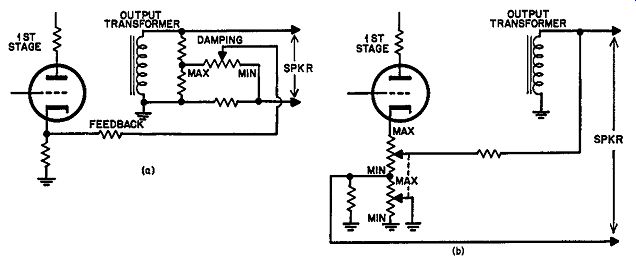
Fig. 325. Two variations of circuit that uses constant total feedback
(assuming nominal loading), but varies the proportions of voltage and
current feedback to change the damping factor.
Fig. 326. Two variations of circuit that uses positive and negative current feedback to adjust the damping factor. a--Uses only one potentiometer. b--Requires only half the series loss to obtain the feedback voltage, by using a two-gang potentiometer.
If the amplifier without overall feedback has a damping factor in the region of unity-that is, source resistance equal to nominal load resistance, then a variation in the current and voltage feed back, which adds up at all times to a total of 20 db, will give a deviation in damping factor from 0.1 to 10. If the amplifier is correctly designed, apart from the damping-factor control, for the use of 20-db overall feedback, the stability criteria and frequency response should be satisfactory. Changing the proportions of feed back by use of a ganged control will give this available variation of damping factor without any other undesirable effects.
The other form of damping-factor control has the questionable advantage that the source resistance can be made negative. Working in terms of source resistance, rather than damping factor, this means that the resistance can be reduced to the zero point, corresponding with infinite damping factor, and then can be further made negative to neutralize some of the voice-coil resistance. This should improve the coupling between the amplifier and the voice coil movement because it is like winding the voice coil with a better conductor than copper or aluminum.
The only simple way to achieve this is to use positive and negative current feedback (Fig. 326). Negative current feedback reduces damping factor or increases the source resistance. Positive current feedback works to a point where the source resistance be comes zero-that is, the output voltage does not change as the load resistance is varied and then, taking the positive feedback a little further, the output resistance even goes negative-putting a load on the amplifier increases the output voltage of the amplifier.
The basic disadvantage is that the stability criteria of the amplifier as a whole cannot possibly be kept constant because the total feedback used in the overall loop cannot be constant. Although the amplifier characteristic can be kept within acceptable tolerances in the audio-frequency range, there may still be peaking at sub- or ultra-sonic frequencies with the attendant distortions that this can produce. The use of positive feedback in this manner over a number of stages also complicates the problem, as mentioned in connection with the use of the "infinite gain" stage.