WHATEVER the audio measurement, there are usually two, three or more ways of making it, dependent upon the equipment you have and upon the personnel doing the job. If it is of a laboratory nature, requiring precision results, one kind of equipment will serve the purpose best, while routine production measurements call for equipment that makes the procedure possible while making minimum demands on the skill of the operator. Within these limits, however, there are variations of method according to purpose and application.
In high-fidelity and other equipment in the audio field, two trends appear. One is toward individual test components that can be put together in a variety of ways to perform a multiplicity of checks; and the other is toward package units which contain everything necessary for audio testing.
The advantages of individual components are their versatility and the fact that they are usually much easier to check in the event of failure of one of the components. With the composite "system checker," the failure of an individual component will often throw out several of the tests for which the equipment is intended and will make it difficult to ascertain just why correct results are not being achieved.
However, the composite system does have the advantage of simplicity in routine use. Most better-class manufacturers prefer to build their own production test equipment to fit in with their own particular schedules. They may use ready-made components built into a composite testing system, or they may build the complete unit from the bottom up.
Audio oscillator
For most of the audio tests you may want to make, you will need an audio sine-wave generator. It is necessary for checking frequency response, measuring power output and almost all tests except those involving some other type of generator, such as a square-wave generator. With modern standards of distortion in audio equipment, it is vital that the audio sine-wave generator itself have low distortion.
But the term "low" can have different connotations according to application. For some purposes and methods of test, a distortion of 2% would be considered low, while for testing a high fidelity amplifier with a rated distortion of 0.1% and using a harmonic-distortion meter, a distortion of 2% would be considered very much too high in an oscillator.
However, there may be another way of making the measurement-using an oscilloscope, for example, that enables an oscillator with, say, 2% distortion to be utilized for checking the distortion of an amplifier producing only 0.1%. But this is rather unconventional and certainly not adapted to routine testing. So for routine applications it is essential that the sine-wave generator have a distortion figure of at least an order of magnitude better than the distortion in the equipment to be tested, otherwise filters will have to be utilized to eliminate the residual harmonics at the input end.
For taking frequency runs the audio sine-wave generator must have a flat frequency response. By this we mean that the output should not vary as the frequency control is rotated. This is sometimes a difficult requirement to meet, although many modern signal generators come pretty close to achieving it. But when making frequency measurements to an accuracy of, say, 0.1 db (which is necessary if the response is specified to within 0.5 db, for example), very few audio sine-wave generators, if any, are good enough without some further method of checking their accuracy.
For most audio test purposes, precision of frequency calibration is not vital to maintain low drift. However, in many measurements drift from the calibration can be disconcerting, to say the least, even though it may not be vital.
Three basic types of audio signal generator are now on the market. These use the heterodyne or beat-frequency principle and two types of R-C feedback. The feedback principle can vary in a number of other ways, but from the viewpoint of overall performance the two types result in a multirange and single-range oscillator, respectively.
With the heterodyne type of oscillator two high frequencies, usually 100 kc or higher, are heterodyned and the audio frequency is the beat-note resultant (Fig. 201). The usual practice is to swing the frequency of the stronger oscillator and maintain a distortionless waveform in the weaker one. This results in the best audio waveform in the output and also gives the best control of frequency to provide a frequency-stable output.
Of course it is necessary to use temperature-compensated components and, if possible, to maintain a reasonably uniform operating temperature in the oscillator itself. Any drift in the high frequencies results in a much bigger percentage drift of the audio-frequency output. The drift is related to the high frequencies rather than to the audio output frequency of the moment. For example, if the high frequencies are 100 kc and the drift is 0.1%, this represents a 100-cycle change. If the audio oscillator swings from 20 cycles to 20 kc, a change of 100 cycles is 0.5% of 20 kc. But it is 500% of 20 cycles! In fact, it will result in the oscillator being difficult to maintain on zero at the low-frequency end.
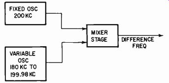
Fig. 201. Basic principle of the heterodyne, or beat frequency, audio oscillator.
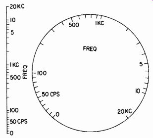
Fig. 202. The scale for a good beat frequency oscillator is logarithmic for
most of its range, but is linear at the bottom end, down to zero.
For this reason an oscillator of this type requires a much better stability than 0.1%. It should maintain its stability to within a cycle or two in the 100-kc fundamental frequencies, otherwise the drift at the low-frequency end will be considerable.
Usually this type of oscillator employs either a variable inductor, with the inductance being changed by some kind of loss arrangement that expands the rate of change at the low end, or else a variable capacitor in which the rate of change of capacitance is expanded over the scale at the low end to produce an approximation to a logarithmic frequency scale, usually from about 100 cycles to the top end of the range (Fig. 202). It is difficult to maintain the logarithmic characteristic right down to, say, 20 cycles. A beat-note oscillator, unlike the other types, goes right down to zero so it cannot be logarithmic to the bottom of its scale. Somewhere there has to be a transition to an approximately linear scale, usually at about 100 cycles.
The use of "zero beat" is a good test of the ability of the oscillator to produce good waveform right down to the lowest wanted frequency, generally 20 cycles. If there is any "pulling" between the fundamental frequencies, due to stray coupling, this will destroy the waveform and also make the zero-beat point indeterminate. The result is a "spread" over which the oscillators will not produce a beat. Also, at a relatively high frequency (say 10 cycles or higher) suddenly a rather poor waveform will appear.
By maintaining good isolation between the fundamental frequencies and using a detector which produces no cross-coupling between the two, the resultant output will maintain good wave form and an accurate zero beat becomes possible within the range of the zero adjustment.
Fig. 203 shows the photo and basic schematic of a well-engineered beat-frequency instrument, using capacitive tuning.
The best way for setting up the correct frequency calibration with the zero adjustment is to use the 60-cycle line frequency to inject a small quantity of a 60 cycle sine-wave from the power supply. This will result in a beat between the 60 cycles produced by the oscillator and the 60 cycles from the line frequency, which can be adjusted to zero. Use care to avoid possible confusion for the oscillator can produce 60 cycles in two places-one on each side of zero. We need to be sure that the 60 cycles obtained is on the right side of zero.
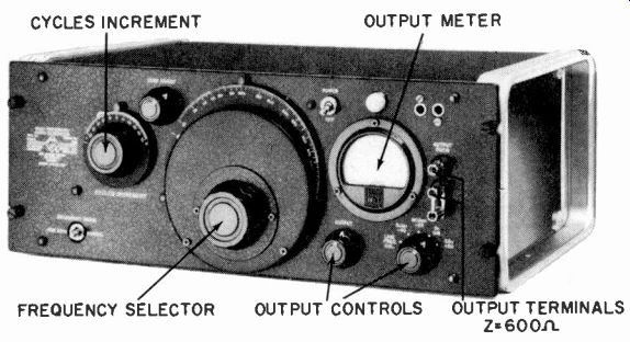
Fig. 203. Front view (above) and basic schematic (below) of beat-frequency
audio oscillator, type 1304-B (Courtesy General Radio Co.)
If it is on the wrong side, then 60 cycles will be an "inversion" of the true 60 cycles. The zero beat will occur at about 120 cycles on the scale and 60 cycles will appear at a scale reading of about 180 cycles. Providing a zero position on the scale makes it easier to zero-adjust the oscillator by turning the ZERO AD JUST until the output needle dips to zero, then adjusting to 60 cycles, switching in the 60-cycle beat and adjusting again to zero beat at this point, taking care not to go through zero. Then the oscillator is accurately set.
Apart from the drift problem, heterodyne oscillators maintain calibration very closely. Once you have set the calibration by this procedure, the percentage error throughout the rest of the scale will be very small. If the error due to line frequency is off, say, 1%, this means the 60 cycle calibration will be 1% off of its true value, but the error at 1,000 cycles will usually be consider ably less than 1% (probably as close as the dial can be read).
This type of instrument has the advantage that the whole audio range is covered in one sweep of the scale. It is difficult to get the low distortion figures obtainable with resistance-capacitance oscillators, however, and 2% is a good figure for a beat-note oscillator. With special care and design the distortion can be reduced to considerably less than 1%, but is liable to increase drastically if the instrument goes out of adjustment in any way.
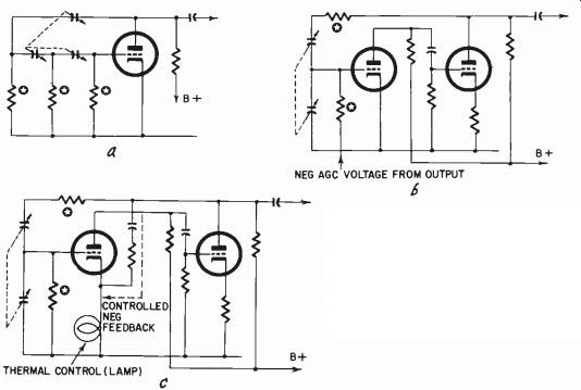
Figs. 204-a,-b-c. Three basic R-C feedback oscillators discussed in the text.
Those resistors marked with a star are frequency deter mining, and could be
made vari able in place of the capacitors shown.
Most R-C oscillators cover the required range in overlapping frequency sweeps of not more than a 10-to-1 ratio. Some increase the precision of their control by utilizing steps of a little more than 3.5 to 1, so two steps are required for each decade of frequency. Most modern R-C oscillators, however, cover just a little more than a decade of frequency, so one sweep of the main dial is necessary to cover each decade of frequency. A little overlap is usually provided, to insure that no frequencies are omitted and to avoid the necessity of switching from one end of the range to the other to see what happens between, say, 190 and 210 cycles, just because 200 cycles is at the opposite end of consecutive ranges.
Modern R-C oscillators achieve very low distortion figures because they utilize both negative and positive feedback. Three basic circuits are shown in Fig. 204. The first is an early one that produces a progressive 180° shift at the frequency of oscillation. The second uses positive feedback with zero shift and automatic bias to control oscillation magnitude. Neither of these has particularly low distortion and the first is subject to drift. The third uses positive and negative feedback, the latter being thermally controlled.
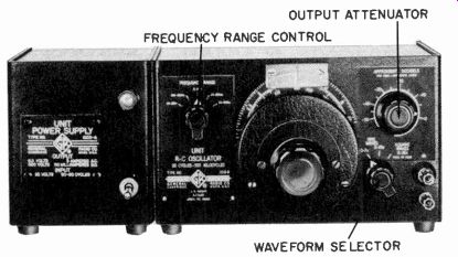
Fig. 205. An R-C oscillator employing the basic circuit of Fig. 204-b. (Courtesy
General Radio Co.)
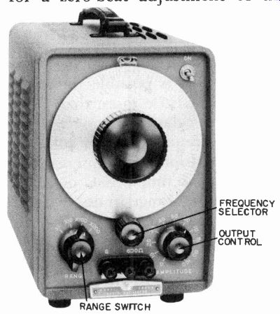
Fig. 206. An R-C oscillator employing the basic circuit of Fig. 204-c. (Courtesy
Hewlett-Packard Co.)
The use of combined feedback (the third circuit of Fig. 204) makes it possible to produce extremely high frequency accuracy, especially when close-tolerance high-stability components are used in the frequency-discriminating elements of the positive feedback circuits and the high negative feedback reduces the harmonic content of the output to any level desired. These facts, together with avoiding the necessity for a zero-beat adjustment of the heterodyne type, have resulted in the great popularity of R-C oscillators in recent years. Figs. 205 and 206 show typical examples.
A comparatively recent development is the "single-sweep" R-C oscillator. This uses the same basic circuitry as Fig. 206 but, instead of using only fixed resistances with variable capacitances (or vice versa) to produce the phase shifts, the fixed elements are combined to make the overall phase-shifting networks combinations of complex impedances. Thus the same multi-gang capacitor, which covers a sweep range of about 10 to 1 in the simpler circuit, covers a sweep range of a little over 1,000 to 1 in this revised circuit. This is illustrated in Fig. 207.
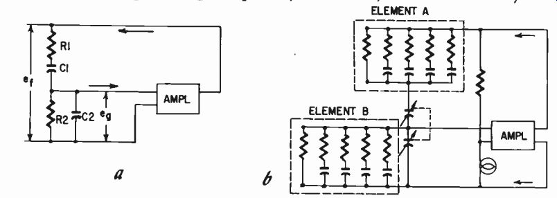
Figs. 207-a,-b. The circuit change necessary to make the R-C oscillator circuit
of Fig. 204-c cover the audio range in a single sweep: (a) simple circuit covering
ranges of 10:1 frequency ratio; (b) as modified to cover a. 1000:1 frequency
ratio.
With the simple arrangement the relationship between the phase-shifting components of a single network is a quadrature one, and the phase angle of both impedances of the voltage divider at the operating frequency is usually at least 45°. By using complex impedances, the phase angle of both impedances of the dividing network is much less than 45° (in the region of 15° or less). Thus, it is possible to make 10-to-1 change in capacitance (or maybe a little more than this) produce the same phase and attenuation relationship over a range of more than a 1,000-to-1 change in frequency (Fig. 208).
The precision of frequency control of this oscillator is not as good as the simple R-C oscillators that cover only about a 10-to-1 frequency range in one sweep. But it avoids the disadvantage of the heterodyne type oscillator which requires periodic zero adjustment. So here we have an oscillator with another kind of characteristic: it does not require zero adjustment to calibrate it at any time, but its precision in frequency calibration is not as close as either the multirange or the heterodyne type (with careful attention to zero setting). Its harmonic generation however, can be consistently as good as the multirange R-C types of better design.
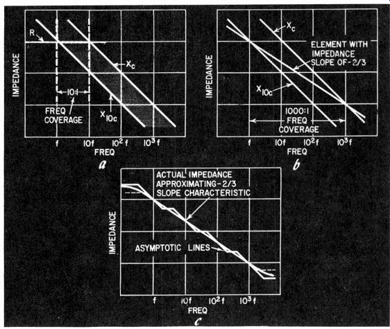
Figs. 208-a,-b-c. Explanation of the development shown in Fig. 207.
At (a) the impedance against which X, is matched is a resistance, and three ranges are needed to cover a 1000:1 ratio; at (b) a theoretical impedance having a slope of -2/3 replaces fixed R, and same capacitance change covers 1000:1 ratio in one range; (c) shows how an impedance with-2/3 slope is synthesized by elements in Fig. 207-b.
Oscillators of this type (Fig. 209) will become popular for routine testing in the near future-testing in which the precision of individual frequencies up and down the scale is not of great importance, but where being able to cover the entire audio range in a single sweep is a valuable time-saving asset. Table 2-1 shows the relative features of audio sine-wave generators.
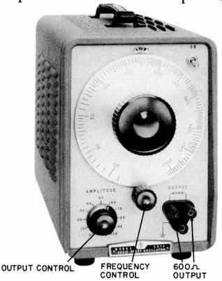
Fig. 209. An R-C oscillator using the method shown in Figs. 207 and 208 to
obtain a 1000:1 cover age in single sweep. (Courtesy Hewlett-Packard Co.)
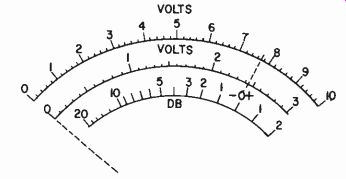
Fig. 210. Scale construction details for an audio voltmeter, using two scales
(0-10 and 0-3) to cover a decade of voltage values.
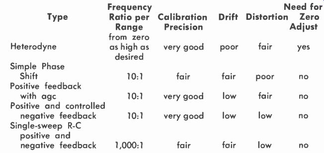
Table 2-1. Characteristics of Various Types of Audio
Vacuum-tube voltmeters
This is a subject that can occupy a complete book on its own in fact it occupies several such books-so we will not devote much space to it here. The requirements of a vacuum-tube voltmeter for audio measurements are similar to those of other test instruments and the ways in which readings can be modified or invalidated by differences in waveform are discussed elsewhere.
What may be discussed in this connection is the difference in types of scale used for different vacuum-tube voltmeters designed for audio measurements.
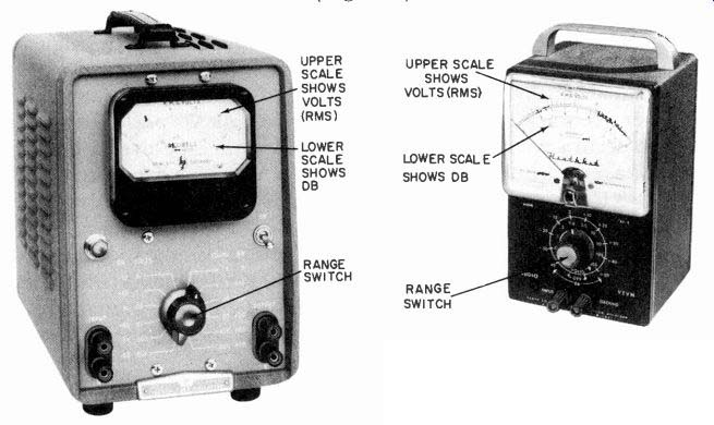
Fig. 211. Two instruments employing the type of scale shown in Fig. 210. (Courtesy
Hewlett Packard Co. and Heath Co).
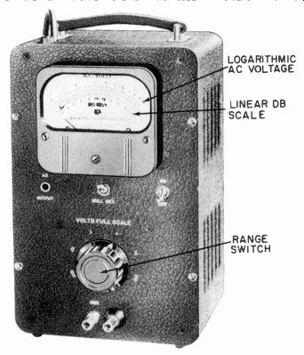
Fig. 212. Audio voltmeter using the special logarithmic scale movement developed
by Stuart Ballantine. (Courtesy Ballantine Laboratories, Inc.).
Some use a basically linear scale, with range switches, generally arranged over half-decade values, so there will be ranges, starting maybe at 10 millivolts full scale, and then 30 my, 100 my, 300 my, 1 volt, 3 volts, 10 volts, etc. This is a very convenient division and usually two scales are arranged so that the difference in reading from one to the next is actually 10 db or a ratio of 3.16 in volts. This means the 10-volt full scale does not coincide exactly with the 3-volt full scale, but the 3 corresponds to about 9.5 volts on the 10-volt scale (Fig. 210). A db scale is included to facilitate references in terms of db. Two examples of this type are shown in Fig. 211.
An alternative form of audio voltmeter utilizes an instrument with a logarithmic scale. This has 1, not 0, at the bottom end of the scale and each range of the instrument covers 20 db, a 10-to-1 ratio. This is achieved by use of a special microammeter with logarithmic scale sensitivity. This type of instrument has the advantage, within the limits of its construction, of providing uniform accuracy in reading over its entire range because 1 db represents the same scale arc whether it is just above the lowest reading the instrument will register or just below the highest (Fig. 212).
Comparing the two types, the linear scale has the advantage of greater accuracy in reading at the top end of the scale only. To attain accuracy comparable to the logarithmic type over a decade of voltages requires two scales, which is why this type uses 0-10 and 0-3 to cover a decade. The logarithmic scale has the advantage of attaining comparable accuracy but only needs half the number of ranges to cover a given scope of levels-a saving in time and frustration. Also the accuracy is uniform, which makes allowance for instrument error easier to visualize. But if you want to read to small fractions of a db, use the linear type and work as near the top of the scale as possible.
Whichever of these types is preferred, its reading is based on a bi-phase rectified signal. The meters are calibrated in the universally accepted rms volts, but this is based on the signal measured being sinusoidal. For no other waveform will the reading given really be rms-in fact, it becomes practically meaningless. To be academic, it might be called a "bi-phase rectified equivalent of sine-wave rms value"! For those few cases where rms readings are important, a true rms meter has been developed using a scale that is logarithmic. However, the scale of this instrument covers only 10 db linearly and then requires a range switch to cover the next power decade. This is necessary only in certain rather specialized applications which will not be considered in this book.
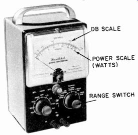
Fig. 213. An audio wattmeter combined with internal and external load switching
to give power readings in watts or db. (Courtesy Heath Company).
A variation of the simple vtvm is the audio wattmeter. This incorporates, into the same instrument, a variety of resistance loads so it measures the power output of the amplifier, providing an internal load for it as well as measuring the voltage output.
One such instrument is shown in Fig. 213. It is particularly helpful on the service bench, where high precision is usually not important but versatility and simplicity of reading count.
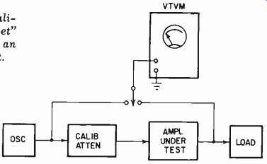
Fig. 214. Method of using a calibrated attenuator, or "gain-set" to
measure the response of an amplifier or other equipment.
Calibrated attenuators
The accepted way of measuring the gain of an amplifier, or any part of an audio system, uses the same vtvm to measure both input and output, and uses the meter on the same range and at the same voltage reading. This means that exactly the same voltage at the same frequency is present at both input and output. To make this possible, a calibrated attenuator is introduced between the input voltage reading and the input to the amplifier or system being measured. The attenuation is then adjusted to attain precisely the same reading at input and output. In this way the insertion loss of the attenuator is equal to the insertion gain of the amplifier.
If the insertion gain of the amplifier is uniform at all frequencies, then the attenuation required in the attenuator--or "gain set" as it is called when provided in a combined instrument--will also be constant. If more attenuation is required to produce the same output, this means the amplifier has more gain at this frequency, and so on.
This method (Fig. 214) appears to be fairly foolproof but it is not as foolproof as it appears. If the components of the gain set are all contained on the same panel, it is possible to get spurious results because of common ground effects between the input and output of the amplifier or system under test which would not occur if complete separation were obtained. These effects may or may not be due to faulty design of the gain set.
As it sometimes requires considerable checking to be sure whether defective performance is due to faulty techniques or components, this setup is ideal where a specific type of equipment is going to be repetitively tested. The test equipment can be bugged out to make sure that the technique and the equipment are functioning properly before the procedure is instituted. Otherwise the best plan is to use a separate attenuator unit of the type shown in Fig. 215, together with separate metering and switching facilities.
Oscilloscopes
The oscilloscope is an almost indispensable instrument for audio measurements. It can be employed to make various measurements instead of merely to supplement or monitor them.
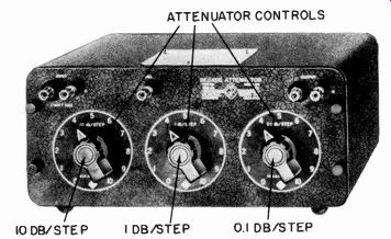
Fig. 215. A convenient type of calibrated attenuator. (Courtesy General Radio
Co.).
The precision of some of the measurement techniques described in this guide rely entirely on the accuracy of the oscilloscope with its attendant deflection amplifiers. This accuracy can, of course, be checked back against itself in the oscilloscope by methods that will be described. But it is always an advantage to have a scope of as high precision as possible. If you want the oscilloscope merely to observe waveforms, then one of the lower-cost ones with average, low-cost deflection amplifiers will probably serve adequately. But if you intend to use it as a measuring instrument in itself, to measure such things as phase angle, harmonic distortion etc., then you should obtain an oscilloscope whose deflection amplifiers are precision-engineered to give calibrated amplification over a specified frequency range with a minimum of phase deviation.
It is advantageous to have a decade-calibrated input attenuator or level switch on both vertical and horizontal input circuits. The calibration signal provided on some oscilloscopes is an asset. It should never be relied upon for instrumental accuracy, but merely be used as a guide.
For low-frequency measurements, a direct-coupled input is necessary as well as the more widely used ac or capacitor-coupled input. Sometimes the equivalent can be achieved by using direct connection to the deflection plate of the cathode-ray tube. For some applications, the best approach is to use an oscilloscope with provision for direct connection, and then use laboratory-standard amplifiers as external deflection amplifiers. Fig. 216 shows a representative high-quality modern scope.
Square-wave generator
A square-wave generator is sometimes specified as an important piece of audio measurement equipment. Actually, by itself it does not tell very much beyond how the equipment being tested performs on square waves. When square-wave testing was first introduced it was pointed out that the behavior of an amplifier on a square wave told more about the overall performance of the amplifier than a simple frequency response.
By merely looking at a square wave of a certain frequency, one could tell what kind of rolloff the amplifier had (whether it was sharp or gradual) and whether it possessed any appreciable phase characteristic of abnormal character. At the same time the square wave was supposed to show the performance of the amplifier on transients. From this statement one might conclude that the square wave does almost as much as all of the previous tests put together.
But this is not quite true.
It does not even properly show all of the information required about the performance of an amplifier on transients, as we shall see later. It does not show anything about distortion characteristics. This means that the sine wave test is still necessary, together with an IM test if so desired, to determine the distortion characteristic of an amplifier.
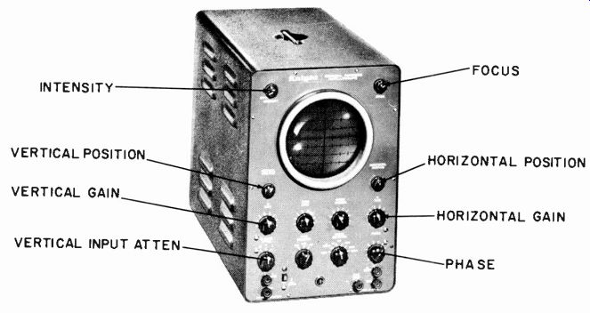
Fig. 216. Typical example of modern oscilloscope suitable for use in audio
measurements. (Courtesy Allied Radio Corp.).
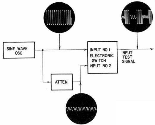
Fig. 217. Using an audio oscillator, attenuator and electronic switch to produce
a "tone-burst" test signal.
If the amplifier has any nonlinearity of its transfer characteristic without associated phase shifts, this cannot show up at all on a square wave. There is no means of knowing whether the velocity of the spot in the vertical part of the wave changes during the traverse. It changes virtually instantaneously from the negative to the positive value--consequently any distortion in this part of the travel does not show up on a square wave.
The horizontal part of the wave presupposes an amplifier in a virtually static condition. The wave should not show any distortion due to the transfer characteristic unless there is a phase, or integrator or differentiator action that causes the part of the waveform that should be horizontal to possess a slope or curvature. Then nonlinear distortion will distort the curvature in this part of the wave. But as this part of the wave now represents another kind of distortion anyway, its utility as part of the square-wave test disappears. One has no means of knowing whether a particular wiggle on a square wave is due to a transient effect in an amplifier or nonlinearity in its transfer characteristic.
However, a square wave is a composite waveform, consisting of a wide range of frequencies, fundamental and harmonic, and as such does provide a 'corm of shock-excited waveform which can test the performance of an amplifier in a way different from separate sine waves. But performance on a square wave is not necessarily any criterion of the amplifier's performance on other kinds of transient-a square wave is a rhythmically repeated transient, which produces a virtually steady state in the amplifier, rather than a "momentary" one as produced by more conventional musical forms.
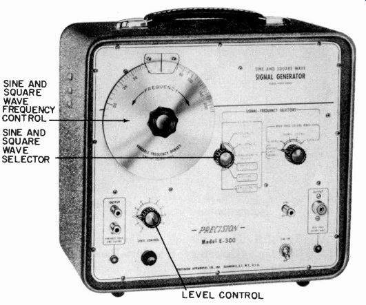
Fig. 218. A combined audio-sine and square-wave generator suitable for service
or technician use. (Courtesy Precision Apparatus Co.)
Nevertheless, exploring the performance of an amplifier with a square wave at the input can be very revealing and therefore an instrument that will produce square waves is quite useful. It is suggested, however, that an electronic switch will also produce square waves and, if the switching frequency is continuously vari able it can be quite as useful as a square-wave generator and provide additional functions. The advantage of an electronic switch over a simple square-wave generator is that it can also square-wave-modulate sine waves to produce the input signal for tone-burst testing using the arrangement shown in Fig. 217.
Another combined instrument that can be quite useful is a sine-wave-square-wave generator (Fig. 218). Probably, for servicing or maintenance purposes, it is more useful than the other combination because the average maintenance engineer will not want to get into tone-burst testing and more complicated things of this nature, but will appreciate the facility of a square wave.
Harmonic-distortion meter
The function of a harmonic-distortion meter is to measure separately the fundamental and harmonic content of any waveform. It does not tell you where the distortion or harmonic originates.
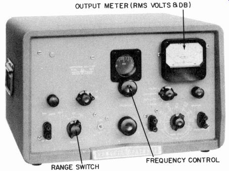
Fig. 219. Example of a harmonic distortion meter. (Courtesy Hewlett-Packard
Co.).
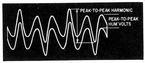
Fig. 220. Method of estimating the relative magnitudes of hum and harmonic
in the measured result of a harmonic meter on a 'scope.
The usual arrangement uses a rejection filter to eliminate the fundamental. This is tunable over a range of frequency so that harmonic-distortion measurements can be made at different fundamental frequencies.
But the distortion meter provides no means of identifying what the residue is. It usually filters the fundamental and leaves frequencies both lower and higher than this. If hum is present below the fundamental frequency, this will register on the indicator as part of the harmonic distortion, just the same as true distortion components. Low-frequency filters can be used to eliminate hum components so the reading obtained is just that due to distortion.
Even then the harmonic-distortion meter tells little of the nature of distortion. But it can be very useful if an output terminal is arranged so that the residue being measured as harmonic distortion can be observed on an oscilloscope. Most harmonic distortion meters make this provision (Fig. 220). Then it is easily possible, by observing the waveform, to determine whether the residue measured is hum or harmonic distortion or partly both. An estimate can be made (Fig. 221) of how much is hum and how much is distortion. At the same time, the distortion can be estimated from the kind of waveform presented, whether it is due to clip ping, to curvature of a second-, third- or other high-order harmonic. Examples of this are illustrated in Fig. 222.
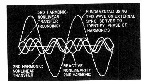
Fig. 221. The 'scope can be used to identify harmonic components of the measured
result on a distortion meter.
As we have just said, the meter merely measures what is present in the waveform. If the reading tells us that the waveform contains 2.5% harmonic, we do not know whether this harmonic is due to the amplifier or whether some of it may already be in the wave form at the input. We can transfer the harmonic-distortion meter to the input of the amplifier and measure the input waveform, if the meter is sensitive enough. Some harmonic-distortion meters are not capable of analyzing waveforms of low enough level to make measurements at the input as well as the output.
But even if the input harmonic measures a little lower than the output harmonic, it can still invalidate the reading. The input reading should be considerably below the level of the output reading for the output reading to have any validity.
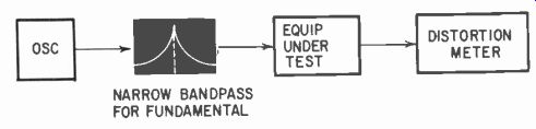
Fig. 222. For really low harmonic measurement, a filter may be needed between
the oscillator and input.
If the harmonic content is of a completely different order-say the input reading is second harmonic, while the output reading [....] balance which provides complete null in the feedback for the fundamental frequency, may cause fluctuations of 10 db or more in the effective forward gain of the stage. This results in increased distortion.
Suppose the maladjustment of the twin-T network yields a null which is 0.5% instead of zero. This means the feedback at the fundamental will be only 46 db less than that at harmonic.
If the feedback at harmonic represents a loop gain of 60 db, then there is a feedback for the fundamental of 14 db, which represents this much attenuation of the fundamental. To produce the required output from the filter five times as much input is needed, which means some of the circuit has to operate at a much higher level than would be the case with zero feedback.
Consequently, although the electronic filter may be designed to operate the tubes under conditions where distortion is 2% or less, it can produce 5% or 10% distortion, and provides a discrimination between the fundamental and distortion of only 46 db. So this 5% to 10% distortion will only be cut by a factor of about 200.
Assuming that the input waveform is pure enough for the purpose, there still remains the manner of presentation of the distortion component in the output waveform and the problem of discovering whether this reading is due to hum or harmonics of the signal. This is determined by interpretation of the oscilloscope trace. For routine distortion measurements, personnel may not be capable of making such interpretations.
What is needed is a throw switch which will give readings on a meter representing the different components.
For this purpose, high- and low-pass filters or rejection filters to eliminate hum frequencies are needed, so the hum frequencies and distortion components can be measured separately.
This is not as difficult a problem as the filters for purifying the fundamental at the input. Here the fundamental is rejected in the distortion meter, so the residue consists of hum frequencies and distortion, both of similar orders of level. Consequently simple filters can readily separate the two and produce independent readings for hum and distortion.
A disadvantage of the harmonic distortion meter is that, even though interpretive measures are used, we have no means of assessing directly the annoyance factor of the harmonics measured.
Second, third or any particular order of harmonic by itself will give an indication which is the true rms value of the difference [...] (or average or whatever designation we like to give to the wave form relationships) between the fundamental and the harmonic in question. Combinations of uniformly distributed harmonics also produce a virtual rms reading within fairly close limits.
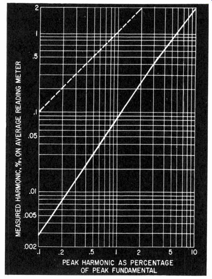
Fig. 224. Readings obtained on a harmonic distortion meter for values of peak
clipping distortion to peak fundamental.
But modern feedback amplifiers are apt to produce orders of distortion that are very low until the clipping point is reached the point at which the amplifier suddenly teases to amplify the input waveform proportionately. This means that the bulk of the input waveform is accurately amplified and only a small portion near each peak is suddenly clipped right off. On a harmonic distortion meter that measures average or rms voltages, this gives a reading that is deceptively low compared with a comparison between the peak harmonic component to the peak fundamental waveform. Fig. 224 is a graph of the correlation between peak relationship and average or rms readings, as given by the average distortion meter.
As clipping on an audio waveform reproduced over a speaker is apt to sound like a separate sound--as if the voice coil were knocking at its end stops--it is not appreciably masked by the fundamental, because .it has a completely different frequency component. This means its annoyance factor can be very much greater than the simple relationship of higher-order harmonics in what may be analyzed as a normal overtone structure. Consequently the peak-to-peak relationship more closely approximates the annoyance factor than does the accepted average or rms relationship.
A method of measuring distortion that compares input against output has been developed by the author, using simple comparative traces on the oscilloscope. This is easily refined by means of fine and coarse resistance balance controls and phase compensation so that quite precise readings can be obtained.
As some operators find difficulty in interpreting readings on an oscilloscope it is suggested that the same principle be applied to the evolution of a simpler distortion meter which is independent of the purity of the input signal. This method compares the output waveform against the input waveform, balancing off a pro portion of the input waveform against the output waveform. It then determines the distortion residue in the output waveform due to the intervening amplifier. This method is illustrated in skeleton form in Fig. 225.
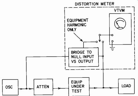
Fig. 225. A suggested modification to the regular distortion meter to Make
it independent of small harmonic content in test oscillator.
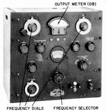
Fig. 226. A two-signal audio genera tor provides signal source for a variety
of IM measurements. (Courtesy General Radio Co.)
Two or three of its features recommend it. One is that the distortion meter does not require a frequency adjustment to balance out the fundamental. Over small ranges of frequency the adjustment for balance of the input waveform does not vary considerably as with the average distortion meter. With the conventional method, if the oscillator drifts at all, the distortion meter begins to show a reading due to the fundamental creeping in. So experimentation on equipment to see the effect on distortion of various circuit changes or adjustments requires continuous adjustment of the conventional distortion meter to balance out the fundamental and make sure that the distortion reading really is just distortion.
Using this recommended method, such a critical balance does not become necessary.
The main feature of the method is that, whether or not the input waveform has a lower distortion component than the expected output waveform, it does not contribute to the reading in the ambiguous manner discussed earlier.
A third advantage is the simplification of the harmonic-distortion meter circuit, reducing the likelihood of the instruments developing errors due to faults in the circuit itself.
A method of measuring distortion preferred for some laboratory purposes uses a wave analyzer to measure the precise magnitude of the fundamental and of each successive harmonic detected. This requires computation-squaring, summing and taking the square root-to obtain an rms value.
Intermodulation test meters
These take quite a variety of forms according to the kind of distortion to be measured, whether it is the sum and difference tones using a low and high frequency, or the difference tone measurement using two high frequencies. Either measurement can be made by using one composite instrument which generates both the required input signals and also performs the analysis on the output signal, or by a collection of instruments that perform the separate functions: for example, the two-sine-wave audio generator (Fig. 226) together with a separate analysis meter for the output; or individual audio signal generators, mixers and the required filters and other components as separate entities can be combined to make the required measurements. The alternative is an instrument that combines the functions in one unit (Fig. 227).
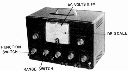
Fig. 227. A common type of composite IM test set. (Courtesy Heath Company).
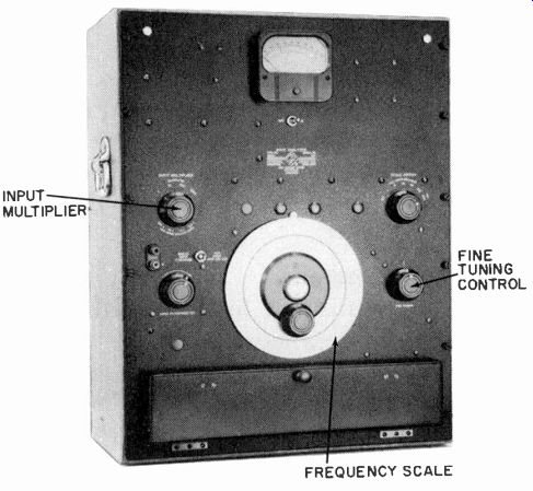
Fig. 228. The well-known wave analyzer uses a crystal gate frequency filter.
(Courtesy General Radio Co.).
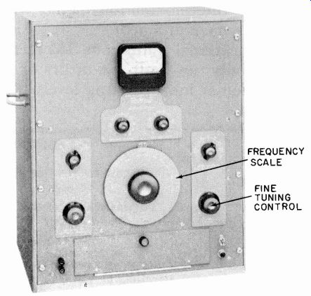
Fig. 229. An alternative circuit uses a feed back frequency filter of adjustable
width. (Courtesy Hewlett-Packard Co.).
The choice of methods will depend on the desired amount of versatility and whether the equipment has to be used for multiple purposes. Either way, the method itself has restrictions as to its usefulness which are noted in the various sections in which IM distortion measurements are discussed.
Intermodulation meters have the advantage-using the first method-that the measurement is not dependent on the purity of either frequency, provided it is reasonably sinusoidal. But the accuracy and significance of the indication are dependent on a number of other factors.
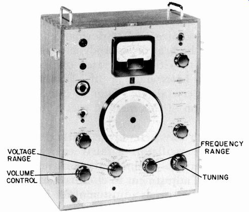
Fig. 230. Another type of wave analyzer uses a direct, adjustable, twin-T
feedback frequency filter, of variable percentage, (rather than cycles) width.
(Courtesy Bruel and Kjoer, Brush Electronics Co.).
Choice of test frequencies can limit the margin for picking up intermodulation products, and the indication produced by any specific frequencies will depend on the filter characteristics. This is why almost no two intermodulation meters will produce the same reading for the same equipment.
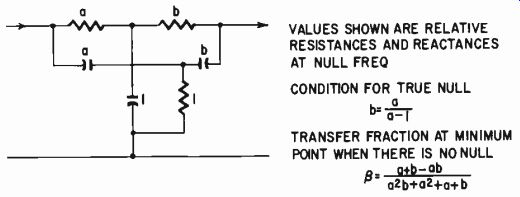
Fig. 231. Relevant quantities for determining the characteristic of a parallel,
or twin-T, filter.
Apart from these functional limitations, IM meters can vary in other respects. Sensitivity can limit the utility of the instrument for measuring distortion at low operating levels. The author considers the principal usefulness of an IM meter is in the development laboratory, where it will tell whether a specific change in an amplifier circuit results in reduced IM distortion. The numerical values measured do not have any absolute significance when compared with similar measurements taken on other instruments.
Wave analyzers
From the laboratory viewpoint, a wave analyzer can be regarded as complementary to a signal generator. This fact shows up in the similarity of circuit choice and performance comparisons. One type corresponds to the beat or heterodyne oscillator. It combines the unknown quantity with a calibrated oscillator and measures the output of a fixed heterodyne or "if." Fig. 228 shows one that uses a very narrow "crystal-gate" filter to channel off the output frequency. A variation of this method uses a feedback type filter (Fig. 229).
The problem with any heterodyne method is similar to that with the heterodyne oscillator: a fairly critical zero-adjustment procedure is necessary to calibrate the instrument. The crystal gate needs additional adjustment to eliminate null-transfer effects, while the feedback filter needs adjustment for both frequency and sharpness. The heterodyne method does have the advantage that the bandwidth, in cycles, can be adjusted over a certain range of sharpness.
Fig. 232. A wave analyzer using third octave filters to cover the audio range.
(Courtesy Bruel and Kjoer, Brush Electronics Co.).
But either heterodyne type produces a response whose band width is a constant (or adjustable) number of cycles. A filter 2 cycles wide, for example, represents 10% of the frequency or a Q of 10, at 20 cycles, and .01% or a Q of 10,000 at 20,000 cycles.
For many purposes it is better to have a bandwidth that is a constant percentage of the operating frequency. A circuit that achieves this and at the same time avoids the zero-adjustment procedure of the heterodyne type has an adjustable-frequency feedback filter (Fig. 230).
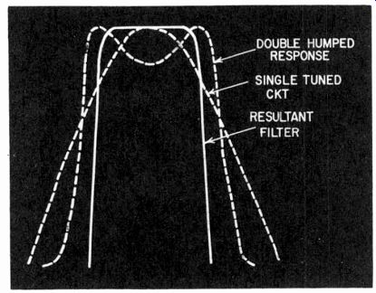
Fig. 233. Synthesis of third octave filters for the analyzer of Fig. 232 is
achieved by combining a single tuned circuit with a double-humped band-pass.
The usual type of feedback filter for this purpose employs a twin-T filter (Fig. 231), which has the property of producing a null at its output for just one frequency. The conventional arrangement uses values in each series limb twice that of the shunt limb. Consequently, 1% components will result in 0.5% balance error if all the components have their maximum error in such a direction as to be additive. Deviation of any one series element by 1% causes the resultant null to be in error by .0625%, while error of one shunt element by 1% causes a resultant error of 0.125%.
As against this, of course, the large amount of negative feedback will magnify these errors by the loop gain factor. Frequency-of-null errors are quite small, which is an advantage. The accuracy of null, and also the sharpness of the resultant frequency response or null, are both dependent on the twin-T working out of virtually zero impedance into an open circuit. Ideally it should work out of and into a cathode follower, with a gain stage sandwiched between.
The use of circuitry which produces appreciable impedance at the input or output results in distortion of the symmetry of the frequency response, due to either the effect of the load on the twin-T output or the effect of the twin-T circuit as a load on the source that feeds it. Serious modification of this nature produces a phase shift which upsets the feedback stability criteria, especially in the vicinity of null.
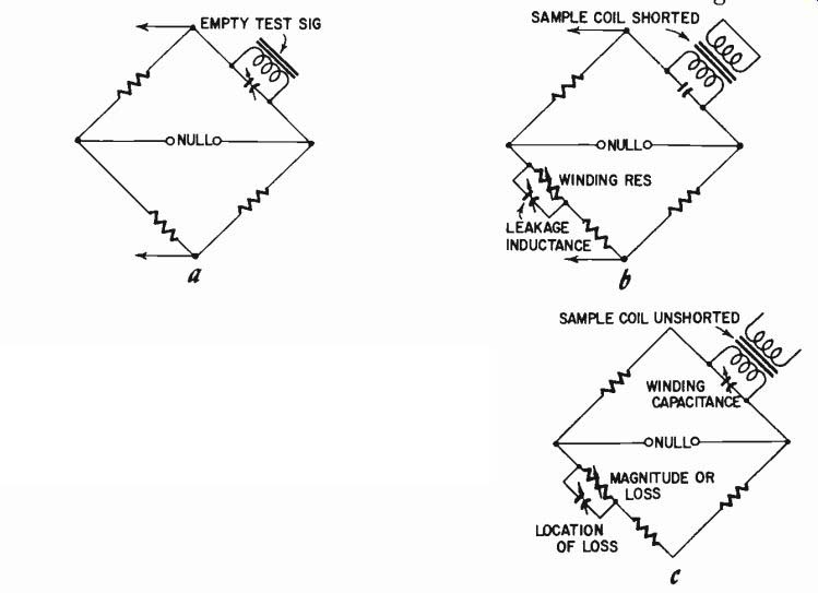
Figs. 234-a,-b,-c. How a bridge circuit can be adapted for special purposes,
in this case for investigating the properties of a coil for an iron-core transformer.
Further variations of this type of circuit use values in which the transfer characteristic of the twin-T either does not go down to zero or true null, and positive feedback, under precision control, which is used to adjust the null point. Sometimes the circuit is arranged to go through a phase reversal instead of a true null, with negative feedback to offset the excess positive feedback that results. Or else a lower basic amplification is used so the effective positive feedback in the vicinity of null increases the gain at this point, while reducing it everywhere else.
Another approach to frequency analysis (for quite different purposes) uses a set bandpass filter to separate the unknown frequency or frequencies into predetermined bands. Fig. 232 shows one using third-octave filters that covers the audio range from 40 cycles to 20 kc in 27 steps. It can be used for making the spectrum-analysis type of presentation, which only identifies components as lying within a certain one-third octave of frequency range. This instrument has L-C type bandpass filters and a single-tuned circuit to "fill in" a double-hump-coupled circuit (Fig. 233).
Flutter and wow meters
Instruments in this class are virtually an adaptation of various FM detector circuits. A constant frequency is applied to a suitable recording, which is played on the device suspected of flutter or wow. The detector then measures any fluctuation in the output frequency, giving a reading in percentage deviation. The principal problems involved in this type of meter concern obtaining satisfactory sensitivity to minute deviations without making the instrument extremely subject to normal and legitimate drifts. In general, a satisfactory instrument falls into the laboratory class and requires a certain amount of skill in handling.
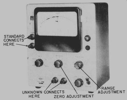
Fig. 235. A deviation bridge, useful in production for selecting components
of any type within desired tolerances. (Courtesy Bruel and Kjoer, Brush Electronics
Co.).
Bridges
Varieties of the basic bridge circuit are used extensively for audio measurements. Apart from those used for measuring basic quantities (described in the next section ) specialized bridge circuits have found application in almost every branch of audio. A modification of the Wien bridge is used in some resistance-capacitance oscillators for feedback.
The great asset of the bridge method of measurement is that careful arrangement can always compensate for or eliminate the effect of extraneous quantities that invalidate other methods. For example, one application is in a particular kind of shorted-turns tester used for laboratory checking of coils for audio application, before their cores are inserted. A bridge technique enables the precise location of a shorted-turns form of loss and the effective cross-section of winding involved, however small (Fig. 234). This arrangement is useful for finding weak spots in winding construction that are difficult to locate by other methods. It also shows up distributed loss effect due to impregnating material interacting with enamel insulation, a state of affairs difficult to detect by normal leakage tests.
For production purposes, it is convenient to have a bridge set up so individual components can be checked for tolerance, especially where close tolerances are necessary. Fig. 235 shows a simple type of ac bridge arranged so that any component can be compared against a standard. The bridge is set up to give a direct reading indication (in percentage) of any deviation from standard.
A useful feature is the easily replaceable scale that enables any desired method of acceptance or rejection to be set up in a minimum of time.
Recommended Reading
1. Rhys Samuel, The V. T. V. M., Gernsback Library Book No. 57, 1956.
2. E. N. Bradley, Radio Servicing Instruments, Norman Price Publishers, 1953.
3. F. E. Terman and J. M. Pettit, Electronic Measurements, McGraw Hill Book Co., 1952.
4. Norman H. Crowhurst, "The Use of Twin-T Networks," Audio Magazine; May, 1958.
5. Darwin H. Harris, "Phase-Shift Oscillator," RADIO-ELECTRONICS Magazine; January, 1954.
6. P. N. Markantes, "Sine- and Square-Wave Generator," RADIO-ELECTRONICS Magazine; May, 1954.
7. Richard Graham, "Compact Wide-Range Oscillator," RADIO Electronics Magazine; July, 1954.
8. John W. Straede, "R-C Controlled Oscillator," RADIO-ELECTRONICS Magazine; December, 1955.
9. "An R-C Oscillator that Covers the 20-cps-20 kc Range in a Single Dial Sweep," Hewlett-Packard Journal; January, 1957.