Listening Test Methodologies and Standards
A number of listening-test methodologies and standards have been developed. They can be followed rigorously, or used as practical guidelines for other testing. In addition, standards for listening-room acoustics have been developed.
Some listening tests can only ascertain whether a codec is perceptually transparent; that is, whether expert listeners can tell a difference between the original and the coded file, using test signals and a variety of music. In an ABX test, the listener is presented with the known A and B sources, and an unknown X source that can be either A or B; the assignment is pseudo-randomly made for each trial. The listener must identify whether X has been assigned to A or B. The test answers the question of whether the listener can hear a difference between A and B. ABX testing cannot be used to conclude that there is no difference; rather, it can show that a difference is heard. Short music examples (perhaps 15 to 20 seconds) can be auditioned repeatedly to identify artifacts. It is useful to analyze ABX test subjects individually, and report the number of subjects who heard a difference.
Other listening tests may be used to estimate the coding margin, or how much the bit rate can be reduced before transparency is lost. Other tests are designed to gauge relative transparency. This is clearly a more difficult task. I f two low lossy codecs both exhibit audible noise and artifacts, only human subjectivity can determine which codec is preferable. Moreover, different listeners may have different preferences in this choice of the lesser of two evils. For example, one listener might be more troubled by bandwidth reduction while another is more annoyed by quantization noise.
Subjective listening tests can be conducted using the ITU-R Recommendation BS.1116-1. This methodology addresses selection of audio materials, performance of playback system, listening environment, assessment of listener expertise, grading scale, and methods of data analysis. For example, to reveal artifacts it is important to use audio materials that stress the algorithm under test.
Moreover, because different algorithms respond differently, a variety of materials is needed, including materials that specifically stress each codec. Selected music must test known weaknesses in a codec to reveal flaws. Generally, music with transient, complex tones, rich in content around the ear's most sensitive region, 1 kHz to 5 kHz, is useful.
Particularly challenging examples such as glockenspiel, castanets, triangle, harpsichord, tambourine, speech, trumpet, and bass guitar are often used.
Critical listening tests must use double-blind methods in which neither the tester nor the listener knows the identities of the selections. For example, in an "A-B-C triple-stimulus, hidden-reference, double-blind" test the listener is presented with a known A uncoded reference signal, and two unknown B and C signals. Each stimulus is a recording of perhaps 10 to 15 seconds in duration. One of the unknown signals is identical to the known reference and the other is the coded signal under test. The assignment is made randomly and changes for each trial. The listener must assign a score to both unknown signals, rating them against the known reference. The listener can listen to any of the stimuli, with repeated hearings. Trials are repeated, and different stimuli are used. Headphones or loudspeakers can be used; sometimes one is more revealing than the other. The playback volume level should be fixed in a particular test for more consistent results. The scale shown in FIG. 24 can be used for scoring. This 5 point impairment scale was devised by the International Radio Consultative Committee (CCIR) and is often used for subjective evaluation of perceptual-coding algorithms.
Panels of expert listeners rate the impairments they hear in codec algorithms on a 41-point continuous scale in categories from 5.0 (transparent) to 1.0 (very annoying impairments).
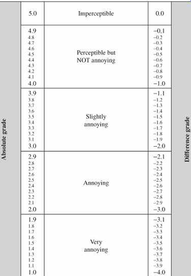
FIG. 24 The subjective quality scale specified by the ITU-R Rec. BS.1116
recommendation. This scale measures small impairments for absolute and differential
grading.
The signal selected by the listener as the hidden reference is given a default score of 5.0. Subtracting the score given to the actual hidden reference from the score given to the impaired coded signal yields the subjective difference grade (SDG). For example, original, uncompressed material may receive an averaged score of 4.8 on the scale. If a codec obtains an average score of 4.8, the SDG is 0 and the codec is said to be transparent (subject to statistical analysis). If a codec is transparent, the bit rate may be reduced to determine the coding margin. A lower SDG score (for example, -2.6) assesses how far from transparency a codec is. Numerous statistical analysis techniques can be used. Perhaps 50 listeners are needed for good statistical results. Higher reduction ratios generally score less well. For example, FIG. 25 shows the results of a listening test evaluating an MPEG-2 AAC main profile codec at 256 kbps, with five full-bandwidth channels.
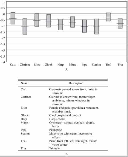
FIG. 25 Results of listening tests for an AAC main profile codec at 256 kbps,
five-channel mode showing mean scores and 95% confidence intervals. A. The
vertical axis shows the AAC grades minus the reference signal grades. B. This
table describes the audio tracks used in this test. (ISO/IEC JTC1/SC29/WG-11
N1420, 1996)
In another double-blind test conducted by Gilbert Soulodre using ITU-R guidelines, the worst-case tracks included a bass clarinet arpeggio, bowed double bass and harpsichord arpeggio (from an EBU SQAM CD), pitch pipe (Dolby recording), Dire Straits (Warner Brothers CD 7599 25264-2 Track 6), and a muted trumpet (University of Miami recording). In this test, when compared against a CD-quality reference, the AAC codec was judged best, followed by PAC, Layer III , AC-3, Layer II , and IT IS codecs, respectively. The highest audio quality was obtained by the AAC codec at 128 kbps and the AC-3 codec at 192 kbps per stereo pair. As expected, each codec performed relatively better at higher bit rates. In comparison to AAC, an increase in bit rate of 32, 64, and 96 kbps per stereo pair was required for PAC, AC-3, and Layer II codecs, respectively, to provide the same audio quality. Other factors such as computational complexity, sensitivity to bit errors, and compatibility to existing systems were not considered in this subjective listening test.
MUSHRA (MUltiple Stimulus with Hidden Reference and Anchors) is an evaluation method used when known impairments exist. This method uses a hidden reference and one or more hidden anchors; an anchor is a stimulus with a known audible limitation. For example, one of the anchors is a lowpass-coded signal. A continuous scale with five divisions is used to grade the stimuli: excellent, good, fair, poor, and bad. MUSHRA is specified in ITU-R BS.1534. Other issues in sound evaluation are described in ITU-T P.800, P.810, and P.830; ITU-R BS.562-3, BS.644-1, BS.1284, BS.1285, and BS.1286, among others.
In addition to listening-test methodology, the ITU-R Recommendation BS.1116-1 standard also describes a reference listening room. The BS.1116-1 specification recommends a floor area of 20 m2 to 60 m2 for monaural and stereo playback and an area of 30 m2 to 70 m2 for multichannel playback. For distribution of low-frequency standing waves, the standard recommends that room dimension ratios meet these three criterion:
1.1(w /h) = (l/h)
= 4.5(w /h) - 4; (w /h) < 3; and (l/h) < 3
where l, w , h are the room's length, width, and height. The 1/3-octave sound pressure level, over a range of 50 Hz to 16,000 Hz, measured at the listening position with pink noise is defined by a standard-response contour. Average room reverberation time is specified to be: 0.25(V/V0) 1/3 where V is the listening room volume and V0 is a reference volume of 100 m3. This reverberation time is further specified to be relatively constant in the frequency range of 200 Hz to 4000 Hz, and to follow allowed variations between 63 Hz and 8000 Hz. Early boundary reflections in the range of 1000 Hz to 8000 Hz that arrive at the listening position within 15 ms must be attenuated by at least 10 dB relative to direct sound from the loudspeakers. It is recommended that the background noise level does not exceed ISO noise rating of NR10, with NR15 as a maximum limit.
The IEC 60268-13 specification (originally IEC 268-13) describes a residential-type listening room for loudspeaker evaluation. The specification is similar to the room described in the BS.1116-1 specification. The 60268-13 specification recommends a floor area of 25 m2 to 40 m2 for monaural and stereo playback and an area of 30 m2 to 45 m2 for multichannel playback. To spatially distribute low frequency standing waves in the room, the specification recommends three criterion for room-dimension ratios:
(w /h) = (l/h) = 4.5(w /h) - 4; (w /h) < 3; and (l/h) < 3
where l, w , h are the room's length, width, and height. The reverberation time (measured according to the ISO 3382 standard in 1/3-octave bands with the room unoccupied) is specified to fall within a range of 0.3 to 0.6 seconds in the frequency range of 200 Hz to 4000 Hz. Alternatively, average reverberation time should be 0.4 second and fall within a frequency contour given in the standard. The ambient noise level should not exceed NR15 (20 dBa to 25 dBA).
The EBU 3276 standard specifies a listening room with a floor area greater than 40 m2 and a volume less than 300 m3. Room-dimension ratios and reverberation time follow the BS.1116-1 specification. In addition, dimension ratios should differ by more than ±5%. Room response measured as a 1/3-octave response with pink noise follows a standard contour.
Listening Test Statistical Evaluation
As Mark Twain and others have said, "There are three kinds of lies: lies, damned lies, and statistics." To be meaningful, and not misleading, interpretation of listening test results must be carefully considered. For example, in an ABX test, if a listener correctly identifies the reference in 12 out of 16 trials, has an audible difference been noted? Statistic analysis provides the answer, or at least an interpretation of it. In this case, because the test is a sampling, we define our results in terms of probability.
Thus, the larger the sampling, the more reliable the result. A central concern is the significance of the results. I f the results are significant, they are due to audible differences.
Otherwise they are due to chance. In an ABX test, a correct score 8 of 16 times indicates that the listener has not heard differences; the score could be arrived at by guessing. A score of 12/16 might indicate an audible difference, but could also be due to chance. To fathom this, we can define a null hypothesis H0 that holds that the result is due to chance, and an alternate hypothesis H1 that holds it is due to an audible difference. The significance level a is the probability that the score is due to chance. The criterion of significance a is the chosen threshold of a that will be accepted. I f a is less than or equal to a then we accept that the probability is high enough to accept the hypothesis that the score is due to an audible difference. The selection of a is arbitrary but a value of 0.05 is often used. Using this formula:
z = (c - 0.5 - np1)/[np1(1 - p1)] 1/2
where
z = standard normal deviate
c = number of correct responses
n = sample size
p1 = proportion of correct responses in a population due to chance alone (p1 = 0.5 in an ABX test)
We see that with a score of 12/16, z = 1.75. Binomial distribution thus yields a significance level of 0.038. The probability of getting a score as high as 12/16 from chance alone (and not from audible differences) is 3.8%. In other words, there is a 3.8% chance that the listener did not hear a difference. However, since a is less than a (0.038 < 0.05) we conclude that the result is significant and there is an audible difference, at least according to how we have selected our criterion of significance. If a is selected to be 0.01, then the same score of 12/16 is not significant and we would conclude that the score is due to chance.
We can also define parameters that characterize the risk that we are wrong in accepting a hypothesis. A Type 1 error risk (also often noted as a ') is the risk of rejecting the null hypothesis when it is actually true. Its value is determined by the criterion of significance; if a = 0.05 then we will be wrong 5% of the time in assuming significant results. Type 2 error risk b defines the risk of accepting the null hypothesis when it is false. Type 2 risk is based on the sample size, value of a, the value of a chance score, and effect size or the smallest score that is meaningful. These values can be used to calculate sample size using the formula:
n = {[z1[p1 (1 - p1)] 1/2 + z2[p2 (1 - p2)] 1/2]/(p2 - p1)} 2
where n = sample size
p1 = proportion of correct responses in a population due to chance alone (p1 = 0.5 in an ABX test)
p2 = effect size: hypothesized proportion of correct responses in a population due to audible differences
z1 = binomial distribution value corresponding to Type 1 error risk
z2 = binomial distribution value corresponding to Type 2 error risk
For example, in an ABX test, if Type 1 risk is 0.05, Type 2 risk is 0.10, and effect size is 0.70, then the sample size should be 50 trials. The smaller the sample size, that is, the number of trials, the greater the error risks. For example, if 32 trials are conducted, a = 0.05, and the effect size is 0.70. To achieve a statistically significance result, a score of 22/32 is needed.
Binomial distribution analysis provides good results when a large number of samples are available. Other types of statistical analyses such as signal detection theory can also be applied to ABX testing. Finally, it is worth noting that statistical analysis can appear impressive, but its results cannot validate a test that is inherently flawed. In other words, we should never be blinded by science.
Lossless Data Compression
The principles of lossless data compression are quite different from those of perceptual lossy coding. Whereas perceptual coding operates mainly on data irrelevancy in the signal, data compression operates strictly on redundancy. Lossless compression yields a smaller coded file that can be used to recover the original signal with bit for-bit accuracy. In other words, although the intermediate stored or transmitted file is smaller, the output file is identical to the input file. There is no change in the bit content, so there is no change in sound quality from coding.
This differs from lossy coding where the output file is irrevocably changed in ways that may or may not be audible.
Some lossless codecs such as MLP (Meridian Lossless Packing) are used for stand-alone audio coding. Some lossy codecs such as MP3 use lossless compression methods such as Huffman coding in the encoder's output stage to further reduce the bit rate after perceptual coding.
In either case, instead of using perceptual analysis, lossless compression examines a signal's entropy.
A newspaper with the headline "Dog Bites Man" might not elicit much attention. However, the headline "Man Bites Dog" might provoke considerable response. The former is commonplace, but the latter rarely happens. From an information standpoint, "Dog Bites Man" contains little information, but "Man Bites Dog" contains a large quantity of information. Generally, the lower the probability of occurrence of an event, the greater the information it contains. Looked at in another way, large amounts of information rarely occur.
The average amount of information occurring over time is called entropy, denoted as H. Looked at in another way, entropy measures an event's randomness and thus measures how much information is needed to describe it.
When each event has the same probability of occurrence, entropy is maximum, and notated as Hmax. Usually, entropy is less than this maximum value. When some events occur more often, entropy is lower. Most functions can be viewed in terms of their entropy. For example, the commodities market has high entropy, whereas the municipal bonds market has much lower entropy. Redundancy in a signal is obtained by subtracting from 1 the ratio of actual entropy to maximum entropy: 1 - (H/Hmax). Adding redundancy increases the data rate; decreasing redundancy decreases the rate: this is data compression, or lossless coding. An ideal compression system removes redundancy, leaving entropy unaffected; entropy determines the average number of bits needed to convey a digital signal. Further, a data set can be compressed by no more than its entropy value multiplied by the number of elements in the data set.
Entropy Coding
Entropy coding (also known as Huffman coding, variable length coding, or optimum coding) is a form of lossless coding that is widely used in both audio and video applications. Entropy coding uses probability of occurrence to code a message. For example, a signal can be analyzed and samples that occur most often are assigned the shortest codewords. Samples that occur less frequently are assigned longer codewords. The decoder contains these assignments and reverses the process. The compression is lossless because no information is lost; the process is completely reversible.
The Morse telegraph code is a simple entropy code.
The most commonly used character in the English language (e) is assigned the shortest code (.), and less frequently used characters (such as z) are assigned longer codes (- - ..). In practice, telegraph operators further improved transmission efficiency by dropping characters during coding and then replacing them during decoding.
The information content remains unchanged. U CN RD THS SNTNCE, thanks to the fact that written English has low entropy; thus its data is readily compressed. Many text and data storage systems use data compression techniques prior to storage on digital media. Similarly, the abbreviations used in text messaging employ the same principles.
Generally, a Huffman code is a noiseless coding method that uses statistical techniques to represent a message with the shortest possible code length. A Huffman code provides coding gain if the symbols to be encoded occur with varying probability. It is an entropy code based on prefixes. To code the most frequent characters with the shortest codewords, the code uses a nonduplicating prefix system so that shorter codewords cannot form the beginning of a longer word. For example, 110 and 11011 cannot both be codewords. The code can thus be uniquely decoded, without loss.
Suppose we wish to transmit information about the arrival status of trains. Given four conditions, on time, late, early, and train wreck, we could use a fixed 2-bit codeword, assigning 00, 01, 10, and 11, respectively. However, a Huffman code considers the frequency of occurrence of source words. We observe that the probability is 0.5 that the train is on time, 0.35 that it is late, 0.125 that it is early, and 0.025 that it has wrecked. These probabilities are used to create a tree structure, with each node being the sum of its inputs, as shown in FIG. 26. Moreover, each branch is assigned a 0 or 1 value; the choice is arbitrary but must be consistent. A unique Huffman code is derived by following the tree from the 1.0 probability branch, back to each source word. For example, the code for early arrival is 110. In this way, a Huffman code is created so that the most probable status is coded with the shortest codeword and the less probable are coded with longer codewords. There is a reduction in the number of bits needed to indicate on time arrival, even though there is an increase in the number of bits needed for two other statuses. Also note that prefixes are not repeated in the codewords.
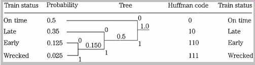
FIG. 26 A Huffman code is based on a nonduplicating prefix, assigning the
shorter codewords to the more frequently occurring events. If trains were usually
on time, the code in this example would be particularly efficient.
The success of the code is gauged by calculating its average code length; it is the summation of each codeword length multiplied by its frequency of occurrence. In this example, the 1-bit word has a probability of 0.5, the 2-bit words have a probability of 0.35, and the 3-bit words have a combined probability of 0.15; thus the average code length is 1(0.5) + 2(0.35) + 3(0.15) = 1.65 bits. This compares favorably with the 2-bit fixed code, and approaches the entropy of the message. A Huffman code is suited for some messages, but only when the frequency of occurrence is known beforehand. I f the relative frequency of occurrence of the source words is approximately equal, the code is not efficient. I f an infrequent source word's probability approaches 1 (becomes frequent), the code will generate coded messages longer than the original. To overcome this, some coding systems use adaptive measures that modify the compression algorithm for more optimal operation. The Huffman code is optimal when all symbols have a probability that is an integral power of one half.
Run-length coding also provides data compression, and is optimal for highly frequent samples. When a data value is repeated over time, it can be coded with a special code that indicates the start and stop of the string. For example, the message 6666 6666 might be coded as 86. This coding is efficient; run-length coding is used in fax machines, for example, and explains why blank sections of a page are transmitted more quickly than densely written sections. Although Huffman and run-length codes are not directly efficient for music coding by themselves, they are used for compression within some lossless and lossy algorithms.
Audio Data Compression
Perceptual lossy coding can provide a considerable reduction in bit rates. However, whether audible or not, the signal is degraded. With lossless data compression, the signal is delivered with bit-for-bit accuracy. However, the decrease in bit rate is more modest. Generally, compression ratios of 1.5:1 to 3.5:1 are possible, depending on the complexity of the data itself. Also, lossless compression algorithms may require greater processing complexity with the attendant coding delay.
Every audio signal contains information. A rare audio sample contains considerable information; a frequently occurring sample has much less. The former is hard to predict while the latter is readily predictable. Similarly, a tonal (sinusoidal) sound has considerable redundancy whereas a nontonal (noise-like) signal has little redundancy.
For example, a quasi-periodic violin tone would differ from an aperiodic cymbal crash. Further, the probability of a certain sample occurring depends on its neighboring samples. Generally, a sample is likely to be close in value to the previous sample. For example, this is true of a low frequency signal. A predictive coder uses previous sample values to predict the current value. The error in the prediction (difference between the actual and predicted values) is transmitted. The decoder forms the same predicted value and adds the error value to form the correct value.
To achieve its goal, data compression inputs a PCM signal and applies processing to more efficiently pack the data content prior to storage or transmission. The efficiency of the packing depends greatly on the content of the signal itself. Specifically, signals with greater redundancy in their PCM coding will allow a higher level of compression. For that reason, a system allowing a variable output bit rate will yield greater efficiency than one with a fixed bit rate. On the other hand, any compression method must observe a system's maximum bit rate and ensure that the threshold is never exceeded even during low-redundancy (hard to compress) passages.
PCM coding at a 20-bit resolution, for example, always results in words that are 20 bits long. A lossless compression algorithm scrutinizes the words for redundancy and then reformats the words to shorter lengths. On decompression, a reverse process restores the original words. Peter Craven and Michael Gerzon suggest the example of a 20-bit word length file representing an undithered 4-kHz sine wave at -50 dB below peak level, sampled at 48 kHz. Moreover, a block of 12 samples is considered, as shown in Table 10.4. The file size is 240 bits. Observation shows that in each sample the four LSBs (least significant bits) are zero; an encoder could document that only the 16 MSBs (most significant bits) will be transmitted or stored. This is easily accomplished by right justifying the data and then coding the shift count.
Furthermore, the 9 MSBs in each sample of this low-level signal are all 1s or 0s; the encoder can simply code 1 of the 9 bits and use it to convey the other missing bits. With these measures, because of the signal's limited dynamic range and resolution, the 20-bit words are conveyed as 8 bit words, resulting in a 60% decrease in data. Note that if the signal were dithered, the dither bit(s) would be conveyed with bit-accuracy by a lossless coder, reducing data efficiency.

TABLE 4 Twelve samples taken from a 20-bit audio file, showing limited
dynamic range and resolution. In this case, simple data compression techniques
can be applied to achieve a 60% decrease in file size. (Craven and Gerzon,
1996)
In practice, a block size of about 500 samples (or 10 ms) may be used, with descriptive information placed in a header file for each block. The block length may vary depending on signal conditions. Generally, because transients will stimulate higher MSBs, longer blocks cannot compress short periods of silence in the block. Shorter blocks will have relatively greater overhead in their headers. Such simple scrutiny may be successful for music with soft passages, but not successful for loud, highly compressed music. Moreover, the peak data rate will not be compressed in either case. In some cases, a data block might contain a few audio peaks. Relatively few high amplitude samples would require long word lengths, while all the other samples would have short word lengths.
Huffman coding (perhaps using a lookup table) can be used to overcome this. The common low-amplitude samples would be coded with short codewords, while the less common high-amplitude samples would be coded with longer codewords. To further improve performance, multiple codeword lookup tables can be established and selected based on the distribution of values in the current block. Audio waveforms tend to follow amplitude statistics that are Laplacian, and appropriate Huffman tables can reduce the bit rate by about 1.5-bit/sample/channel compared to a simple word-length reduction scheme.
A predictive strategy can yield greater coding efficiency.
In the previous example, the 16-bit numbers have decimal values of +67, +97, +102, +79, +35, -18, -67, -97, -102, -79, -35, and +18. The differences between successive samples are +30, +5, -23, -44, -53, -49, -30, -5, +23, +44, and +53. A coder could transmit the first value of +67 and then the subsequent differences between samples; because the differences are smaller than the sample values themselves, shorter word lengths (7 bits instead of 8) are needed. This coding can be achieved with a simple predictive encode-decode strategy as shown in FIG. 27 where the symbol z-1 denotes a one-sample delay. If the value +67 has been previously entered, and the next input value is +97, the previous sample value of +67 is used as the predicted value of the current sample, the prediction error becomes +30, which is transmitted. The decoder accepts the value of +30 and adds it to the previous value of +67 to reproduce the current value of +97.
FIG. 27 A first-order predictive encode/decode process conveys differences between successive samples.
This improves coding efficiency because the differences are smaller than the values themselves. (Craven and Gerzon, 1996) The goal of a prediction coder is to predict the next sample as accurately as possible, and thus minimize the number of bits needed to transmit the prediction error. To achieve this, the frequency response of the encoder should be the inverse of the spectrum of the input signal, yielding a difference signal with a flat or white spectrum. To provide greater efficiency, the one-sample delay element in the predictor coder can be replaced by more advanced general prediction filters. The coder with a one-sample delay is a digital differentiator with a transfer function of (1 - z-1). An nth order predictor yields a transfer function of (1 - z-1) n, where n = 0 transmits the original value, n = 1 transmits the difference between successive samples, n = 2 transmits the difference of the difference, and so on.
Each higher-order integer coefficient produces an upward filter slope of 6, 12, and 18 dB/octave. Analysis shows that n = 4 may be optimal, yielding a maximum difference of 10.
However, the high-frequency content in audio signals limits the order of the predictor. The high-frequency component of the quantization noise is increased by higher-order predictors; thus a value of n = 3 is probably the limit for audio signals. But if the signal had mainly high-frequency content (such as from noise shaping), even an n = 1 value could increase the coded data rate. Thus, a coder must dynamically monitor the signal content and select a predictive strategy and filter order that is most suitable, including the option of bypassing its own coding, to minimize the output bit rate. For example, an autocorrelation method using the Levinson-Durbin algorithm could be used to adapt the predictor's order, to yield the lowest total bit rate.
A coder must also consider the effect of data errors.
Because of the recirculation, an error in a transmitted sample would propagate through a block and possibly increase, even causing the decoder to lose synchronization with the encoder. To prevent artifacts, audible or otherwise, an encoder must sense uncorrected errors and mute its output. In many applications, while overall reduction in bit rate is important, limitation of peak bit rate may be even more vital. An audio signal such as a cymbal crash, with high energy at high frequencies, may allow only slight reduction (perhaps 1 or 2 bits/sample/channel). Higher sampling frequencies will allow greater overall reduction and peak reduction because of the relatively little energy at the higher portion of the band. To further ensure peak limits, a buffer could be used. Still, the peak limit could be exceeded with some kinds of music, necessitating the shortening of word length or other processing.
The simple integer coefficient predictors described above provide upward slopes that are not always a good (inverse) match for the spectra of real audio signals. The spectrum of the difference signal is thus nonflat, requiring more bits for coding. Every 6-dB reduction in the level of the transmitted signal reduces its bit rate by 1 bit/sample.
More successful coding can be achieved with more sophisticated prediction filters using, for example, noninteger-coefficient filters in the prediction loop. The transmitted signal must be quantized to an integer number of LSB steps to achieve a fixed bit rate. However, with noninteger coefficients, the output has a fractional value of LSBs. To quantize the prediction signal, the architecture shown in FIG. 28 may be employed. The decoder restores the original signal values by simply quantizing the output.
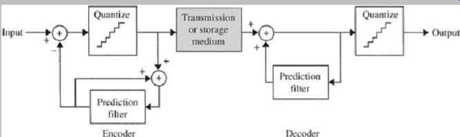
FIG. 28 Noninteger-coefficient filters can be used in a prediction encoder/decoder.
The prediction signal is quantized to an integer number of LSB steps. (Craven
and Gerzon, 1996)
Different filters can be used to create a variety of equalization curves for the prediction error signal, to match different signal spectral characteristics. Different 3rd-order IIR filters, when applied to different signal conditions, may provide bit-rate reduction ranging from 2 to 4 bits, even in cases where the bit rate would be increased with simple integer predictors. Higher-order filters increase the amount of overhead data such as state variables that must be transmitted with each block to the decoder; this argues for lower-order filters. It can also be argued that IIR filters are more appropriate than FIR filters because they can more easily achieve the variations found in music spectra. On the other hand, to preserve bit accuracy, it is vital that the filter computations in any decoder match those in any encoder.
Any rounding errors, for example, could affect bit accuracy.
In that respect, because IIR computation is more sensitive to rounding errors, the use of IIR predictor filters demands greater care.
Because most music spectral content continually varies, filter selection must be re-evaluated for each new block.
Using some means, the signal's spectral content must be analyzed, and the most appropriate filter employed, by either creating a new filter characteristic or selecting one from a library of existing possibilities. Information identifying the encoding filter must be conveyed to the decoder, increasing the overhead bit rate. Clearly, processing complexity and data overhead must be weighed against coding efficiency.
As noted, lossless compression is effective at very high sampling frequencies in which the audio content at the upper frequency ranges of the audio band is low. Bit accuracy across the wide audio band is ensured, but very high-frequency information comprising only dither and quantization noise can be more efficiently coded. Craven and Gerzon estimate that whereas increasing the sampling rate of an unpacked file from 64 kHz to 96 kHz would increase the bit rate by 50%, a packed file would increase the bit rate by only 15%. Moreover, low-frequency effects channels do not require special handling; the packing will ensure a low bit rate for its low-frequency content. Very generally, at a given sampling frequency, the bit-rate reduction achieved is proportional to the input word length and is greater for low-precision signals. For example, if the average bit reduction is 9 bits/sample/channel, then a 16 bit PCM signal is coded as 7 bits (56% reduction), a 20-bit signal as 11 bits (45% reduction), and a 24-bit signal as 15 bits (37.5% reduction). Very generally, each additional bit of precision in the input signal adds a bit to the word length of the packed signal.
At the encoder's output, the difference signal data can be Huffman-coded and transmitted as main data along with overhead information. While it would be possible to hardwire filter coefficients into the encoder and decoder, it may be more expedient to explicitly transmit filter coefficients along with the data. In this way, improvements can be made in filter selection in the encoder, while retaining compatibility with existing decoders.
As with lossy codecs, lossless codecs can take advantage of interchannel correlations in stereo and multichannel recordings. For example, a codec might code the left channel, and frame-adaptively code either the right channel or the difference between the right and left channels, depending on which yields the highest coding gain. More efficiently, stereo prediction methods use previous samples from both channels to optimize the prediction.
Because no psychoacoustic principles such as masking are used in lossless coding, practical development of transparent codecs is relatively much simpler. For example, subjective testing is not needed. Transparency is inherent in the lossless codec. However, as with any digital processing system, other aspects such as timing and jitter must be carefully engineered.