|
|
IIR Filters
The general difference equation contains y(n) components that contribute to the output value. These are feedback elements that are delayed by a unit of time i, and describe a recursive filter. The feedback elements are described in the denominator of the transfer function. Because the roots cause H(z) to be undefined, certain feedback could cause the filter to be unstable. The poles contribute an exponential sequence to each pole's impulse response. When the output is fed back to the input, the output in theory will never reach zero; this allows the impulse to be infinite in duration.
This type of filter is known as an infinite impulse response (IIR) filter.
Feedback provides a powerful method for recalling past samples. For example, an exponential time-average filter adds the current input sample to the last output (as opposed to the previous sample) and divides the result by 2. The equation describing its operation is:
y(n) = x(n) + 0.5y(n - 1).
This yields an exponentially decaying response in which each next output sample is one-half the previous sample value. The filter is called an infinite impulse response filter because of its infinite memory. In theory, the impulse response of an IIR filter lasts for an infinite time; its response never decays to zero. This type of filter is equivalent to an infinitely long FIR filter where:
y(n) = x(n) + 0.5x(n - 1) + 0.25x(n - 2) + 0.125x(n - 3)+ …. +(0.5) Mx(n - M)
In other words, the filter adds one-half the current sample, one-fourth the previous sample, and so on. The impulse response of a practical FIR filter decays exponentially, but it has a finite length, thus cannot decay to zero.
In general, an IIR filter can be described as:
y(n) = ax(n) + by(n - 1)
When the value of b is increased relative to a, the lowpass filtering is augmented; that is, the cutoff frequency is lowered. The value of b must always be less than unity or the filter will become unstable; the signal level will increase and overflow will result.
An IIR filter can have both poles and zeros, can introduce phase shift, and can be unstable if one or more poles lie on or outside the unit circle. Generally, an all-pole filter is an IIR filter. IIR filters cannot achieve linear phase (the impulse response is asymmetrical) except in the case when all poles in the transfer function lie on the unit circle. This is realized when the filter consists of a number of cascaded first-order sections. Because the output of an IIR is fed back as an input (with a scaling element), it is called a recursive filter. An IIR filter always has a recursive structure, but filters with a recursive structure are not always IIR filters.
Any feedback loop must contain a delay element.
Otherwise, the value of a sample would have to be known before it is calculated-an impossibility.
Consider the IIR filter described by the equation:
y(n) = x(n) - x(n - 2) - 0.25y(n - 2)
It can be rewritten as:
y(n) + 0.25y(n - 2) = x(n) - x(n - 2)
Transformation to the z-plane yields:
Y(z) + 0.25z-2Y(z) = X(z) - z-2X(z)
The transfer function is:
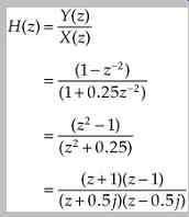
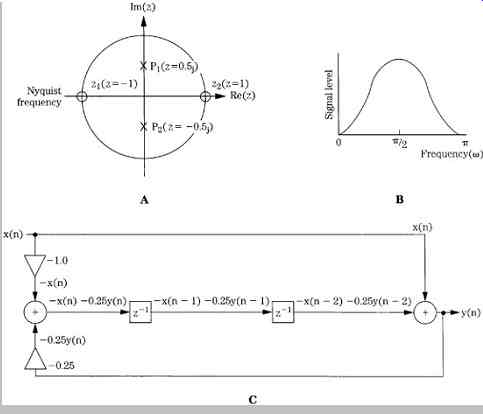
FIG. 13 An example showing the response and structure of a digital bandpass
IIR filter. A. The pole and zero locations of the filter in the z-plane. B.
The frequency response of the filter. C. Structure of the bandpass filter.
There are zeros at z = ±1 and conjugate poles on the imaginary axis at z = ±0.5j, as shown in FIG. 13A. The frequency response can be graphically determined by dividing the product of zero-vector magnitudes by the product of the pole-vector magnitudes; (phase response is the difference between the sum of their angles). The resulting bandpass frequency response is shown in Fig. 17.13B. A realization of the filter is shown in FIG. 13C.
Delay elements have been combined to simplify the design. Similarly, the difference equation:
y(n) = x(n) + x(n - 2) + 0.25y(n - 2)
... is also an IIR filter. The development of its pole/zero plot, frequency response, and realization are left to the ambition of the reader.
In general, it is easier to design FIR filters with linear phase and stable operation than IIR filters with the same characteristics. However, IIR filters can achieve a steeper roll-off than an FIR filter for a given number of coefficients.
FIR filters require more stages, and hence greater computation, to achieve the same result. As with any digital processing circuit, noise must be considered. A filter's type, topology, arithmetic, and coefficient values all determine whether meaningful error will be introduced. For example, the exponential time-average filter described above will generate considerable error if the value of b is set close to unity, for a low cutoff frequency.
Filter Applications
An example of second-order analog filter is shown in Fig. 14A, and an IIR filter is shown in FIG. 14B; this is a biquadratic filter section. Coefficients determine the filter's response; in this example, with appropriate selection of the five multiplication coefficients, highpass, lowpass, bandpass, and shelving filters can be obtained. A digital audio processor might have several of these sections at its disposal. By providing a number of presets, users can easily select frequency response, bandwidth, and phase response of a filter. In this respect, a digital filter is more flexible than an analog filter that has relatively limited operating parameters. However, a digital filter requires considerable computation, particularly in the case of swept equalization. As the center frequency is moved, new coefficients must be calculated-not a trivial task. To avoid quantization effects (sometimes called zipper noise), filter coefficients and amplitude scaling coefficients must be updated at a theoretical rate equal to the sampling rate; in practice, an update rate equal to one-half or one-fourth the sampling rate is sufficient. To accomplish even this, coefficients are often obtained through linear interpolation.
The range must be limited to ensure that filter poles do not momentarily pass outside the unit circle, causing transient instability.
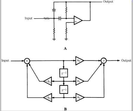
FIG. 14 A comparison of second-order analog and digital filters. A. A second-order
analog filter. B. An IIR biquadratic second-order filter section.
Adaptive filters automatically adjust their parameters according to optimization criteria. They do not have fixed coefficients; instead, values are calculated during operation. Adaptive filters thus consist of a filter section and a control unit used to calculate coefficients. Often, the algorithm used to compute coefficients attempts to minimize the difference between the output signal and a reference signal. In general, any filter type can be used, but in practice, adaptive filters often use a transversal structure as well as lattice and ladder structures. Adaptive filters are used for applications such as echo and noise cancellers, adaptive line equalizers, and prediction.
A transversal filter is an FIR filter in which the output value depends on both the input value and a number of previous input values held in memory. Inputs are multiplied by coefficients and summed by an adder at the output. Only the input values are stored in delay elements; there are no feedback networks; hence it is an example of a nonrecursive filter. As described in Section 4, this architecture is used extensively to implement lowpass filtering with oversampling.
In practice, digital oversampling filters often use a cascade of FIR filters, designed so the sampling rate of each filter is a power of 2 higher than the previous filter. The number of delay blocks (tap length) in the FIR filter determines the passband flatness, transition band slope, and stopband rejection; there are M + 1 taps in a filter with M delay blocks. Many digital filters are dedicated chips.
However, general purpose DSP chips can be used to run custom filter programs.
The block diagram of a dedicated digital filter (oversampling) chip is shown in FIG. 15. It demonstrates the practical implementation of DSP techniques. A central processor performs computation while peripheral circuits accomplish input/output and other functions. The filter's characteristic is determined by the coefficients stored in ROM; the multiplier/accumulator performs the essential arithmetic operations; the shifter manages data during multiplication; the RAM stores intermediate computation results; a microprogram stored in ROM controls the filter's operation. The coefficient word length determines filter accuracy and stopband attenuation. A filter can have, for example, 293 taps and a 22-bit coefficient; this would yield a passband that is flat to within ±0.00001 dB, with a stopband suppression greater than 120 dB. Word length of the audio data increases during multiplication; truncation would result in quantization error thus the data must be rounded or dithered. Noise shaping can be applied at the accumulator, using an IIR filter to redistribute the noise power, primarily placing it outside the audio band. Noise shaping is discussed in Section 18.
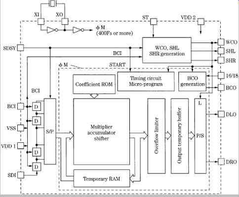
FIG. 15 An example showing the functional elements of a dedicated digital
filter (oversampling) chip.
Sources of Errors and Digital Dither
Unless precautions are taken, the DSP computation required to process an audio signal can add noise and distortion to the signal. In general, errors in digital processors can be classified as coefficient, limit cycle, overflow, truncation, and round-off errors. Coefficient errors occur when a coefficient is not specified with sufficient accuracy. For example, a resolution of 24 bits or more is required for computations on 16-bit audio samples. Limit cycle error might occur when a signal is removed from a filter, leaving a decaying sum. This decay might become zero or might oscillate at a constant amplitude, a condition known as limit cycle oscillation. This effect can be eliminated, for example, by offsetting the filter's output so that truncation always produces a zero output.
Overflow occurs when a register length is exceeded, resulting in a computational error. In the case of wraparound, when a 1 is added to the maximum value positive two's complement number, the result is the maximum value negative number. In short, the information has overflowed into a nonexistent bit. The drastic change in the amplitude of the output waveform would yield a loud pop if applied to a loudspeaker. To prevent this, saturating arithmetic can be used so that when the addition of two positive numbers would result in a negative number, the maximum positive sum is substituted instead. This results in clipping-a more satisfactory, or at least more benign, alternative. Alternatively, designers must provide sufficient digital headroom.
Truncation and round-off errors occur whenever the word length of a computed result is limited. Errors accumulate both inside the processor during calculation, and when word length is reduced for output through a D/A converter.
However, A/D conversion always results in quantization error, and computation error can appear in different guises.
For example, when two n-bit numbers are multiplied, the number of output bits will be 2n - 1. Thus, multiplication almost doubles the number of bits required to represent the output. Although many hardware multipliers can perform double-precision computation, a finite word length must be maintained following multiplication, thus limiting precision.
Discarded data results in an error analogous to that of A/D quantization. To be properly modeled, multiplication must be followed by quantization; multiplication does not introduce error, but inability to keep the extra bits does. It is important to note that unnecessary cumulative dithering should be avoided in interim calculations.
Rather than truncate a word, for example, following multiplication, the value can be rounded; that is, the word is taken to the nearest available value. This results in a peak error of 1/2 LSB, and an rms value of 1/(12) 1/2, or 0.288 LSB. This round-off error will accumulate over successive calculations. In general, the number of calculations must be large for significant error to occur. However, in addition, dither information can be lost during computation. For example, when a properly dithered 16-bit word is input to a 32-bit processor, even though computation is of high precision, the output signal might be truncated to 16 bits for conversion through the output D/A converter. For example, a 16-bit signal that is delayed and scaled by a 12-dB attenuation would result in a 12-bit undithered signal. To overcome this, digital dithering to the resolution of the next processing (or recording) stage should be used in a computation.
To apply digital dithering, a pseudo-random number of the appropriate magnitude is added to each sample and then the new LSB is rounded up or down to the nearest quantization interval according to value of the portion to be discarded. In other words, a logical 1 is added to the new LSB and the lower portion is discarded, or the lower portion is simply discarded. The lower bit information thus modulates the new LSB and provides the linearizing benefit of dithering. A different pseudo-random number is used for each audio channel. To duplicate the effects of analog dither, two's complement digital dither values should be used to provide a bipolar signal with an average zero value.
In some cases, noise shaping is also applied at this stage.
Bipolar pseudo-random noise and a D/A converter can be used to generate analog dither.
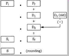
FIG. 16 An example of digital redithering used during a truncation or rounding
computation. (Vanderkooy and Lipshitz, 1989)
As an example of digital dithering, consider a 20-bit resolution signal that must be dithered to 16 bits. IIR and noise-shaping filters with digital feedback can exhibit limit cycle oscillations with low-level signals if gain reduction or certain equalization processing (resulting in gain changes) is performed; digital dither can be used to randomize these cycles.
John Vanderkooy and Stanley Lipshitz have shown that truncated or rounded digital words can be redithered with rectangular pdf or triangular pdf fractional numbers, as shown in FIG. 16. A rectangular pdf dither word D1 is added to a digital audio word with integer part Pi and fractional part Pf . The carry bit dithers the rounding process in the same way that 1 LSB analog rectangular pdf dither affects an A/D converter. When a statistically independent rectangular pdf dither D2 is added, triangular pdf dither results. This triangular pdf dither noise power is Q2/6 and rounding noise power is Q2/12 so the total noise power is Q2/4. The final sum has integer part Si and fractional part Sf , which become S upon rounding.
In cases of gain fading, triangular pdf appears to be a better choice than rectangular pdf because it eliminates noise modulation as well as distortion, at the expense of a slightly higher noise floor. To minimize audibility of this noise penalty, highpass triangular pdf dither can be most appropriate in rounding. The triangular pdf statistics are not changed. However, dither samples are correlated. Average dither noise power is Q2/6, with no noise at 0 Hz and double the average value at the Nyquist frequency. Hence the term: highpass dither. This shaping becomes more pronounced with noise increasingly shifted outside the audio band, as the oversampling ratio is increased, for example, by eight times. The audible effect of a noise penalty is lessened when oversampling is used because in band noise is relatively decreased proportional to the oversampling rate. Further reduction of the Q2/12 requantization noise power can be achieved through noise shaping circuits, as described in Section 18.
As noted, the problem of error sources is applicable to both audio samples as well as the computations used to determine other system operators, such as filter coefficients. For example, improperly computed filter coefficients could shift the locations of poles and zeros, thus altering the characteristics of the response. In some cases, an insufficiently defined coefficient can cause a stable IIR filter to become unstable. On the other hand, the quantization of filter coefficients will not affect the linear operation of a circuit, or introduce artifacts that are affected by the input signal or that vary with time. The effect of coefficient errors in a filter is generally determined by the number of coefficients determining the location of each pole and zero. The fewer the coefficients, the lower the sensitivity. However, when poles and zeros are placed in locations where they are few, the effect of errors is greater.
DSP Integrated Circuits
A DSP chip is a specialized hardware device that performs digital signal processing under the control of software algorithms. DSP chips are stand-alone processors, often independent of host CPUs (central processing units), and are specially designed for operations used in spectral and numerical applications. For example, large numbers of multiplications are possible, as well as special addressing modes such as bit-reverse and circular addressing. When memory and input/output circuits are added, the result is an integrated digital signal processor. Such a general purpose DSP chip is software programmable, and thus can be used for a variety of signal-processing applications. Alternatively, a custom signal processor can be designed to accomplish a specific task.
Digital audio applications require long word lengths and high operating speeds. To prevent distortion from rounding error, the internal word length must be 8 to 16 bits longer than the external word. In other words, for high-quality applications, internal processing of 24 to 32 bits or more is required. For example, a 24-bit DSP chip might require a 56-bit accumulator to prevent overflow when computing long convolution sums.
Processor Architecture
DSP chips often use a pipelining architecture so that several instructions can be paralleled. For example, with pipelining, a fetch (fetch instruction from memory and update program counter), decode (decode instruction and generate operand address), read (read operand from memory), and execute (perform necessary operations) can be effectively executed in one clock cycle. A pipeline manager, aided by proficient user programming, helps ensure efficient processing.
DSP chips, like all computers, are composed of input and output devices, an arithmetic logic unit, a control unit, and memory, interconnected by buses. All computers originally used a single sequential bus (von Neumann architecture), shared by data, memory addresses, and instructions. However, in a DSP chip a particularly large number of operations must be performed quickly for real time operation. Thus, parallel bus structures are used (such as the Harvard architecture) that store data and instructions in separate memories and transfer them via separate buses. For example, a chip can have separate buses for program, data, and direct memory access (DMA), providing parallel program fetches, data reads, as well as DMA operations with slower peripherals.
A block diagram of a general purpose DSP chip is shown in FIG. 17; many DSP chips follow a similar architecture. The chip has seven components: multiply accumulate unit, data address generator, data RAM, coefficient RAM, coefficient address generator, program control unit, and program ROM. Three buses interconnect these components: data bus, coefficient bus, and control bus. In this example, the multiplier is asymmetrical; it multiplies 24-bit sample words by 12-bit coefficient words.
The result of multiplication is carried out to 36 bits. For dynamic compression, the 12-bit words containing control information are derived from the signal itself; two words could be taken together to provide double precision when necessary. A 40-bit adder is used in this example. This adds the results of multiplications to other results stored in the 40-bit accumulator. Following addition in the arithmetic logic unit (ALU), words must be quantized to 24 bits before being placed on the data bus. Different methods of quantization can be applied.
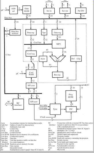
FIG. 17 Block diagram of a digital signal processor chip. The section surrounded
by a dashed line is the arithmetic unit where computation occurs. Independent
buses are used for data, coefficients, and control.
Coefficients are taken from the coefficient RAM, loaded with values appropriate to the task at hand, and applied to the coefficient bus. Twenty-four-bit data samples are moved from the data bus to two data registers. Parallel and serial inputs and outputs, and data memory can be connected to the data bus. This short memory (64 words by 24 bits, in this case) performs the elementary delay operation. As noted, to speed multiple multiplications, pipelining is provided. Necessary subsequent data is fed to intermediate registers simultaneously with operations performed on current data.
Fixed Point and Floating Point
DSP chips are designed according to two arithmetic types, fixed point and floating point, which define the format of the data they operate on. Fixed-point (or fixed-integer) chips use two's complement, binary integer data. Floating-point chips use integer and floating-point numbers (represented as a mantissa and exponent). The dynamic range of a fixed-point chip is based on its word length. Data must be scaled to prevent overflow; this can increase programming complexity. The scientific notation used in a floating-point chip allows a larger dynamic range, without overflow problems. However, the resolution of floating point representation is limited by the word length of the exponent.
Many factors are considered by programmers when deciding which DSP chip to use in an application. These include cost, programmability, ease of implementation, support, availability of useful software, availability of internal legacy software, time to market, marketing impact (for example, the customer's perception of 24-bit versus 32 bit), and sound quality. As Brent Karley notes, programming style and techniques are both critical to the sound quality of a given audio implementation. Moreover, the hardware platform can also affect sound quality. Neither can be ignored when developing high-quality DSP programs. The Motorola DSP56xxx series of processors is an example of a fixed-point architecture, and the Analog Devices SHARC series is an example of a floating-point architecture. Conventional personal computer processors can perform both kinds of calculations.
Three principal processor types are widely used in DSP-based audio products: 24-bit fixed point, 32-bit fixed point, and 32-bit floating point (24 mantissa bits with 8 exponent bits). Each variant of precision and architecture has advantages and disadvantages for sound quality.
When comparing 32-bit fixed and 24-bit fixed, with the same program running on two DSP chips of the same architecture, the higher precision DSP will obviously provide higher quality audio. However, DSP chips often do not use the same architecture and do not support the same implementation of any given algorithm. It is thus possible for a 24-bit fixed-point DSP chip to exceed the sound quality of a 32-bit fixed-point chip. For example, some DSP chips have hardware accelerators that can off-load some processing chores to free up processing resources that can be allocated to audio quality improvements or extra features. Programming methods such as double-precision arithmetic and truncation-reduction methods may be implemented to improve quality. Optimization programming methods can be performed on any of the available DSP architectures, but are often not implemented (or only in limited numbers) because of processing or memory limitations.
For higher-quality audio implementations, a 24-bit fixed point DSP chip can implement double-precision filtering or processing in strategic components of a given algorithm to improve the sound quality beyond that of a 32-bit fixed point DSP chip. The combination of two 24-bit numbers into one 48-bit integer allows very high-fidelity processing.
This is possible in some cases due to the higher processing power available in some 24-bit DSP chips over less efficient 32-bit DSP chips. Some manufacturers carefully hand-optimize their implementations to exceed the sound quality of competitors using 32-bit fixed-point DSP chips. Chip manufacturers often provide different versions of audio decoders and audio algorithms with and without qualitative optimizations to allow the customer to evaluate cost versus quality. In some double-precision 24-bit programming, some high-order bits are used for dynamic headroom, low-order "guard bits" store fractional values, and the balance represent the audio sample; a division of 8/32/8 might be used. In some cases, products with 24-bit chips using double-precision arithmetic are advertised as having "48-bit DSP." As discussed below, performance is also affected by the nature of the instruction set used in the DSP chip.
The comparison of fixed-point and floating-point processors is not straightforward. Generally, in fixed-point processors, there is a trade-off between round-off error and dynamic range. In floating-point processors, computation error is equivalent to the error in the multiplying coefficients.
Floating-point DSP chips offer ease of programmability (they are more easily programmed in a higher-level language such as C++) and extended dynamic range. For example, in a floating-point chip, digital filters can be realized without concern for scaling in state variables.
However, code that is generated in a higher-level language is sometimes not efficiently implemented due to the difference in hand assembly versus C++ compilers. This wastes processing resources that could be used for qualitative improvements. The dynamic range of a 24-bit fixed-point DSP chip is 144 dB and a 32-bit fixed-point chip provides 196 dB, as shown in FIG. 18. In contrast, a 32-bit floating-point DSP chip provides a theoretical dynamic range of 1536 dB. A 1536-dB dynamic range is not a direct advantage for audio applications, but the noise floor is maintained at a level correspondingly below the audio signal. If resources permit, improvements can be implemented in 32-bit floating-point DSP chips to raise the audio quality. The Motorola DSP563xx is an example of a 24-bit fixed-point chip, and the Texas Instruments TMS320C67xx is an example of a 32-bit floating-point chip.
Both platform and programming are critical to the audio quality capabilities of DSP software. Bit length, while an important component, is not the only variable determining audio-quality capabilities. With proper programming, both fixed-point and floating-point processors can provide outstanding sound quality. If needed, optimization programming methods such as double-precision filtering can improve this further.
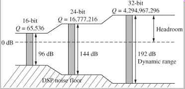
FIG. 18 The dynamic range of fixed-point DSP chips is directly based on their
word length. In some applications, double precision increases the effective
dynamic range.
The IEEE 752 floating-point standard allows either 32 bit single precision (24-bit mantissa and 8-bit exponent) or double precision (64-bit with a 52-bit mantissa and 11-bit exponent). The latter allows very high-fidelity processing, but is not available on all DSP chips.
DSP Programming
As with all software programming, DSP programming allows the creation of applications with tremendous power and flexibility. The execution of software instructions is accomplished by the DSP chip using audio samples as the input signal. Although the architecture of a DSP chip determines its theoretical processing capabilities, performance is also affected by the structure and diversity of its instruction set.
DSP chips use assembly language programming, which is highly efficient. Higher-level languages (such as C++) are easy to use, document, debug, and are independent of hardware. However, they are less efficient and thus slower to execute, and do not take advantage of specialized chip hardware. Assembly languages are more efficient. They execute faster, require less memory, and take advantage of special hardware functions. However, they are more difficult to program, read, debug, are hardware-dependent, and are labor-intensive.
An assembly language program for a specific DSP chip type is written using the commands in the chip's instruction set. These instructions take advantage of the chip's specialized signal processing functions. Generally, there are four types of instructions: arithmetic, program control, memory access and transfer, and input/output. Instructions are programmed with mnemonics that identify the instruction, and reference a data field to be operated upon.
Because many DSP chips operate within a host environment, user front-end programs are written in higher level languages, reserving assembly language programming for the critical audio processing tasks.
An operation that is central to DSP programming is the multiply-accumulate command, often called MAC. Many algorithms call for two numbers to be multiplied, and the result summed with a previous operation. DSP chips feature a multiply-accumulate command that moves two numbers into position, multiplies them together, and accumulates the result, with rounding, all in one operation.
To perform this efficiently, the arithmetic unit contains a multiplier-accumulator combination (see FIG. 17). This can calculate one subproduct and simultaneously add a previous subproduct to a sum, in one machine cycle. To accommodate this, DSP chips rely on a hardware multiplier to execute the multiply-accumulate operation.
Operations such as sum of products and iterative operations can be performed efficiently.
In most cases, the success of a DSP application depends on the talents of the human programmer. Software development costs are usually much greater than the hardware itself. In many cases, manufacturers supply libraries of functions such as FFTs, filters, and windows that are common to many DSP applications. To assist the development process, various software development tools are employed. A text editor is used to write and modify assembly language source code. An assembler program translates assembly language source code into object code. A compiler translates programs written in higher-level languages into object code. A linker combines assembled and compiled object programs with library routines and creates executable object code. The assembler and compiler use the special processing features of the DSP chip wherever possible. A simulator is used to emulate code on a host computer before running it on DSP hardware. A debugger is used to perform low-level debugging of DSP programs. In addition, DSP operating systems are available, providing programming environments similar to those used by general purpose processors.
Filter Programming
DSP chips can perform many signal processing tasks, but digital filtering is central to many applications. As an example of assembly language programming, consider the FIR transversal filter shown in FIG. 19A. It can be described with this difference equation:
y(n) = x(n - 4)h(4) + x(n - 3)h(3) + x(n - 2)h(2) + x(n - 1)h(1) + x(n)h(0)
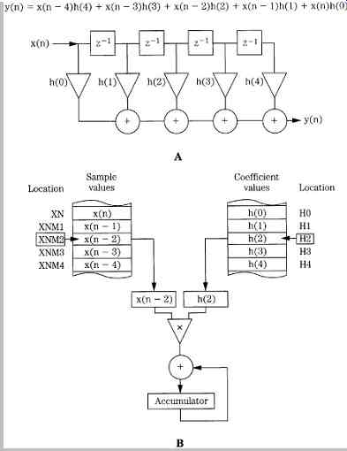
FIG. 19 A five-coefficient FIR filter can be realized with assembly language
code authored for a commercial DSP chip. A. Structure of the FIR filter. B.
Audio sample and filter coefficient values stored in memory are multiplied
and accumulated to form the output samples.
The five input audio sample values, five coefficients describing the impulse response at five sample times, and the output audio sample value will be stored in memory locations; data value x(n) will be stored in memory location XN; x(n - 1) in XNM1; y(n) in YN; h(0) in H0, and so on.
The running total will be stored in the accumulator, as shown in FIG. 19B. In this case, intermediate calculations are held in the T register.
Also see related article: Digital Filters and DSP