We now move from the Construction phase to the Testing Phase...
TEST EQUIPMENT PRINCIPLES
A fully equipped electronic workshop has the entire gamut of test gear from spectrum analyzers and oscilloscopes to insulation testers, variable power supplies, and component analyzers.
Sooner or later, you will have to bite the bullet and buy some test equipment. Your purchase might range from a used moving-coil meter found at an amateur radio fair to a shiny new digital phosphor oscilloscope. Either way, your money is a finite resource and you will want maximum bang per buck.
In this Section, we will investigate how each instrument works, enabling us to understand its inevitable limitations thus putting us in a position to judge which features are worth paying for, and which can be neglected.
The moving coil meter and DC measurements
All test equipment needs some form of indicator to display the results of the measurement. In the tube era, the choice was between a moving coil meter or a cathode ray tube (CRT).
Since CRTs and their necessary support circuitry were (and still are) expensive, the vast majority of test equipment used a moving coil meter. This has two significant consequences. Firstly, it is fashionable for modern studio and consumer audio equipment to be styled to look ''retro'', using hexagonal black bakelite knobs and round black meters having gothic pointers and cream scales. Secondly, there are lots of second-hand moving coil meters available for peanuts.
How a moving coil meter works
If we place one magnet near another, they will leap together so that their unlike poles touch (North to South). Conversely, if we try to force like poles together (North to North, or South to South), they repel. When we pass a current through a wire, it generates a weak magnetic field, and if we wind the wire into a tight coil, this concentrates the magnetic field. The coil is then known as an electromagnet because electricity is used to pro duce the magnetic field. Unsurprisingly, the strength of the electromagnet is proportional to the number of turns and the current flowing.
If we were to place the electromagnet near a permanent magnet, it would be attracted or repelled with a force proportional to the current and, if we could measure this force, we would effectively have measured the current. Moving coil meters use the force to extend a spring, and because the extension of a spring is proportional to the force (Hooke's Law), a scale that actually measures extension can be calibrated in units of current.
It is quite difficult to make a low-friction linear bearing (one that moves in a straight line), but a low-friction rotating bearing is easily made. Unfortunately, although we did not mention it earlier, the attraction and repulsion between the electromagnet and permanent magnet are inversely proportional to the square of the distance between them, resulting in a scale cramped in some sectors but unnecessarily expanded in others. Ideally, we would like a scale with equal-sized graduations throughout its range. Fortunately, shaping the permanent magnet so that it applies a constant radial magnetic field at all positions of the rotating electromagnet produces a linear scale (see FIG.1).
We now have an instrument whose pointer deflection is directly proportional to the current flowing through the coil.
We can make the meter more sensitive by winding more turns of finer wire on the electromagnet, using a more powerful permanent magnet, or weakening the spring. In practice, it is difficult to make a robust meter that requires less than 50 mA for full scale deflection (FSD), and 1mA FSD meters are particularly common.
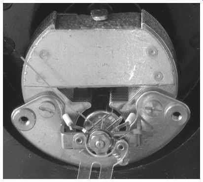
FIG.1 Internal view of moving coil meter (Note the shape of the pole
pieces to produce a radial magnetic field.)
Measuring larger currents
A manufacturer could make different meters to measure different currents, but it is much cheaper to make a standard meter movement and adapt it to measure larger currents. Sup pose that we need a 100mA meter, perhaps for monitoring current in an output tube. Our meter movement still only needs its design current, perhaps 1mA, to drive its pointer to full scale, so we must bypass, or shunt, 99mA away from the delicate meter movement (see FIG.2).
Our problem is to determine the correct value of shunt resistor that will allow 100mA of total current to be shared correctly between the meter (1mA) and the shunt resistor (99mA).
Fortunately, now that we have stated the problem, the solution is quite easy. The meter's internal resistance and electrical sensitivity are usually stated at the bottom of the scale plate, even if the scale itself is calibrated in foot/Lamberts per fortnight.
If we know the current passing through a known resistance, we can use Ohm's law to calculate the voltage developed across that resistance. As an example, suppose that our 1mA movement has an internal (coil) resistance of 65 ohm:
V = IR = 0.001A x 65 ohm = 65mV
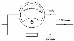
FIG.2 Converting a 0-1mA meter to read 100mA
The shunt resistor is in parallel, so it sees exactly the same voltage as the meter, and if we want to shunt 99mA, we simply use Ohm's law to find the required resistance:
R = V/I = 0.657 Ohm
Sadly, this calculation demonstrates two important points.
Firstly, there is no hope of the required resistor being a standard value, and secondly, the resistor is such a low value that the resistance of its wires becomes critical. Fortunately, this is a sufficiently common application that dedicated meter shunts may be available, or a reasonably close value can itself be shunted by another resistor until the correct value is obtained.
One solution would be to use five 3.3-ohm resistors in parallel (0.66 ohm), and trim this combination with a 500 Ohm variable resistor in parallel.
Measuring small resistances (<10 ohm) accurately is difficult, so it is better to set up a test circuit to pass the required 100mA (perhaps measured by a reliable DVM), and finely adjust the shunt resistance until the meter reads full scale. Nevertheless, adapting a meter to measure different currents is always awkward.
What to do if your meter is unspecified
If you are very unlucky, your meter might not specify its sensitivity and internal resistance. Sensitivity can be found by placing it in series with a variable resistor in series with a reliable DVM set to read current, all connected across a battery. Gently reduce the value of the variable resistor from 100 kOhm until the meter reads precisely full scale, then read off the current measured by the reliable DVM (see FIG.3).
The internal resistance could be found using the resistance range of the DVM, but they tend to sink rather a lot of current, and that might damage the meter under test. A safer method is to leave the variable resistor set to cause FSD, but move the DVM to measure the voltage across the meter under test, and use Ohm's law to calculate its internal resistance (see FIG.4).
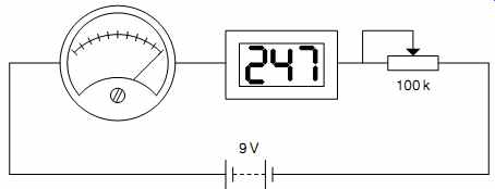
FIG.3 Determining the sensitivity of an unknown meter
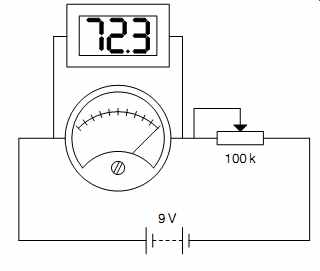
FIG.4 Determining the internal resistance of an unknown meter
As an example, perhaps the first test required 247 mA to attain FSD and when the DVM was used to measure meter voltage, 72.3mV was seen across the meter at FSD.
Rinternal = V/I= 293 Ohm
Measuring voltages
Moving coil meters can be very easily adapted to measure voltages. We know the required current to drive the meter's pointer to FSD, and we know the voltage that we want to cause FSD, so we apply Ohm's law. Perhaps we want to convert our 1mA meter movement to read 40V FSD:
R = V/I = 40V/1mA = 40 kOhm
This calculation effectively states that a 40 k-ohm resistor would pass 1mA if 40V were applied across its terminals. If we placed a perfect 1mA meter in series with the 40 k-ohm resistor, it would achieve FSD when 40V was applied. You will notice that the final voltmeter has an FSD of 40V and a resistance of 40 kOhm, or 1 kOhmper volt. It is common for multimeters to specify their loading resistance in this manner because it allows the user to easily assess the loading, the meter imposes on any given voltage range (see FIG.5).
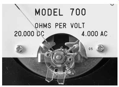
FIG.5 Multimeters often specify their sensitivity in Ohm/V on their scale
plate
But all meters have internal resistance, and our example 1mA meter has an internal resistance of 65 Ohm, so we ought to subtract this from the series resistor to make the total resistance 40 kOhm:
Rseries = 40 kOhm – 65 Ohm = 39.935 kOhm
A freshly calibrated laboratory standard moving coil meter with a 5" mirror scale could attain an accuracy at FSD of +-0.5%, or to put it another way, there is little point in worrying about precisely trimming the series resistance by 0.16% when the meter itself contributes a greater error. The author simply picks suitable theoretical resistor values from his stock of 1% preferred values and doesn't even bother measuring them.
If this attitude offends your sensibilities, consider why we are fitting the meter in the first place. We very rarely measure to confirm a theoretical value - we generally make a measurement to display aberrations from the required value. In short, we want to know if the voltage/current is not what it should be. As an example, car manufacturers do not provide a precisely calibrated 0-15V voltmeter, but simply show red (rather than green) to warn that the battery voltage is not what is ought to be. Once the required value is observably wrong, the precision of the measurement is irrelevant. Distinguishing between the need to identify a fault condition rather than making a precision laboratory measurement is important because it makes identifying fault conditions much cheaper.
Measuring output stage cathode current
It is often necessary to measure an output tube's cathode current. This can be done by inserting a 1-ohm resistor in the cathode circuit and measuring the voltage across it. Postage stamp-sized DVMs tend to be 200mV FSD, and 1mA though a 1-ohm resistor produces 1mV, so these meters can be connected directly across the 1-ohm resistor to give a reading scaled in mA.
We don't need to use a powerful 1-ohm resistor for current sensing and it's actually a disadvantage to do so. The current sense resistor needs precision and fragility, so a 1 ohm, 1% 0.6Wmetal film resistor is ideal because it allows a reasonably accurate measurement, is almost non-inductive, and might serve as a fuse in the event of catastrophic failure. However, +-0.1% DVMs are cheap, so it seems a shame to throw away that accuracy with a 1% sense resistor. In a push-pull amplifier, the balance of output currents is more important than their absolute value, so we need matched 1-ohm resistors.
Matching low-value resistors
1-ohm resistors can't be measured reliably using a DVM because the resistance of the DVM leads is typically 0.2 Ohm and variable contact resistance makes it difficult to make a measurement.
However, matched low-value resistors can be found by soldering a chain of them in series and applying a constant voltage from a regulated power supply across the far ends. Then, using a DVM, measure and record the voltage drop across each resistor and pick resistors with the same measured voltage drop. Accuracy can be improved by:
-- Rather than applying a constant voltage across the ends of the chain, drive a constant current through the chain using the constant current regulator described later in this Section, and power this combination from a regulated voltage.
Because the constant current regulator has a constant voltage across it, it is far more able to maintain a constant current.
-- Before making the first measurement, adjust the voltage or current to give a reading on your DVM that is just under that required to make it change range. For a 3 1/2 digit DVM, 180mV is a good voltage, because it will read 180.0mV, whereas 200mV is a poor choice because it would read 200mV, which is less precise (fewer significant figures).
Matching high-value resistors
Although the bridge was actually invented by Samuel Hunter Christie, this circuit is often known as a Wheatstone bridge because Sir Charles Wheatstone found so many uses for it.
However, Wheatstone did invent the concertina, or accordion, which is perhaps less forgivable.
We have a pair of equal value resistors on the right hand side and an upper resistor on the left hand side to which we want to find a matching lower resistor. If the ratio of upper to lower resistor on each side is identical, the meter will measure 0V. If not, the imbalance will cause a voltage, which can be recorded.
Resistors with equal imbalance voltage are matched to one another, but not necessarily to the upper resistor. This is a very sensitive test, and allows a cheap 31 2 digit DVM set to its 200mV range to easily match resistors to 0.01%.
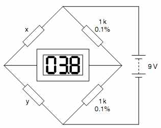
FIG.6 This simple bridge circuit enables precision comparison of resistors.
We can match 1% high-value resistors (>500 ohm) fairly well simply by measuring their resistance with a DVM. Matching 0.1% resistors is trickier. One way would simply be to buy a more accurate DVM. But 41 2 digit DVMs with 0.05% accuracy, or better, are expensive. A much cheaper way is to make a bridge (see FIG.6).
If we want to be able to match to a specific resistor, we need the right hand resistors in the bridge to be perfectly matched. Using the previous method, we can find a pair of perfectly matched resistors, and substitute them into the right hand side of the bridge. These reference resistors should be manufactured for low temperature coefficient, so they will probably be 0.1% metal film, or perhaps even 0.01% metal foil. Because the meter measures ratios, rather than an absolute voltage, power supply voltage is not critical, and the bridge can even be powered by a 9V battery.
Meters and AC measurements
A moving coil meter can only respond to DC, so to measure AC, a rectifier must be added to convert the AC to DC. But AC waveforms can be of any shape, and we are not always able to view them on an oscilloscope, so we need a means of describing important parameters. Once we know the different ways of describing AC, we can choose the rectifier that delivers the measurement we need.
Peak voltages
A convenient way to specify complex waveforms is by peak voltages (see FIG.7).
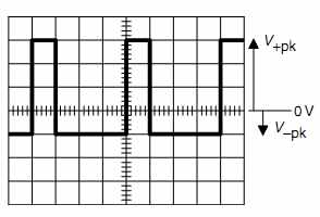
FIG.7 Measuring peak voltages relative to 0 V
Note that because the waveform is asymmetric about 0V, it is necessary to specify V +pk and V -pk separately. In this example, the vertical scale is 1V/div, so V +pk =3V, and V -pk = -1V.
If required, V[pk-pk] could be specified. This could be measured directly as 4Vpk_pk, or it could be calculated from the previous measurements:
Vpk-pk = V +pk – V -pk = +3V – (-)1V = 4V
Vpk and Vpk-pk are particularly useful measures when testing a stage for overload because the numbers directly correlate with the numbers predicted by load lines on a tube's anode characteristics, making it easy to check theory against practice.
Mean level
It is often useful to know the average, or mean level (either voltage or current) of an AC waveform. Since the waveform is assumed to be repetitive, the mean level is determined by finding the mean of one cycle of the waveform.
Conventionally, to find a mean, we sum individual data and divide by the number of items of data. Because an oscilloscope display is a graph of voltage against time, we sum voltages multiplied by their time (producing area) and divide by the total time of the waveform's cycle (see FIG.8).
Note that although this waveform has exactly the same shape as the previous one, V +pk =4V and V -pk =0V. Over one cycle:
First unit of time: V= +4V
Second unit: V=0V
Third unit: V=0V
Fourth unit: V=0V
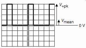
FIG.8 Mean voltage can be intuitively seen because it is proportional
to the area under the waveform. Equal areas above and below 0 V would force
Vmean =0V
We want to find the mean of four data items, so:
Vmean = [4V x 1 + 0V x 3]/4 = 1V
We have calculated the mean level over one cycle of a waveform and assigned it a fixed value, which implies that it is unchanging. If the waveform is repetitive, each cycle is the same as the last, so the mean level must also be constant from one cycle to the next, and it must therefore be a DC voltage (or current).
Any waveform may be considered to be an AC component riding on a constant level of DC known as the DC component (Vmean).
When a single triode stage distorts, it produces predominately 2nd harmonic distortion, and a side effect of this is that it changes the mean level of the signal. A cathode-biased stage typically uses a resistor bypassed by a capacitor, and the capacitor integrates the audio signal to produce a voltage that is partly determined by the mean level of the applied audio. The significance of this is that if we had an accurate DVM, but didn't have a means of directly measuring distortion, we could infer distortion by measuring the change in the DC voltage across the capacitor with and without the signal applied.
Later, we will find that mean level crops up in all sorts of odd places.
Power and RMS
It is often necessary to be able to determine the heating power that a waveform would dissipate in a resistor using P=V^2 /R or P=I^2 R. For DC, this is simply a matter of measuring the appropriate quantities and performing the calculation.
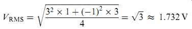
For AC, we need a means of specifying amplitude such that the previous power equations give the correct power. This new value is known as “root of the mean of the squares”, which refers to the way it is calculated. It is invariably abbreviated to RMS or VRMS.
For this example, we have reverted to our original waveform, which we could now describe as having a 4Vpk-pk AC component, but zero DC component. Because the DC component is zero, the waveform has dropped down the oscilloscope screen so that part of it swings negatively (see FIG.9).
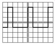
FIG.9 RMS voltage: No intuitive result is possible simply by viewing
the waveform
We calculate VRMS in a very similar way to Vmean, but we first square each voltage, find the mean (of the squares), and finally take the square root of this mean.
Fortunately, we rarely have to calculate Vmean or VRMS manually because a digital oscilloscope is really an application-specific computer in disguise, so it is ideally suited to performing hideous number crunching in the twinkling of an eye (see FIG.10).
The slight discrepancy in Vmean and VRMS measured by the oscilloscope compared to the calculated values simply reflects the author's inability to set the controls precisely on his rather cheap (but perfectly adequate) function generator.
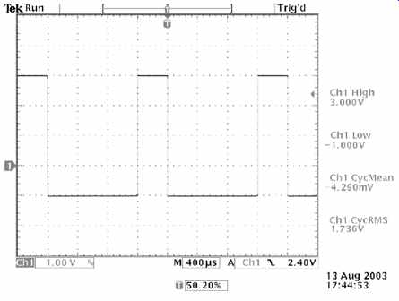
FIG.10 Oscilloscope automated measurements. Wonderful!
Some waveforms such as the sine wave are used so often that conversion factors have been calculated for determining VRMS when Vpk is known. For the sine wave only:
V_RMS = Vpk / √2
The most obvious use of VRMS is in determining the output power of an amplifier from a measurement of voltage across a known load resistance, but since we are only concerned with undistorted output power, a mean reading meter calibrated RMS sine wave is perfectly acceptable. A simple moving coil meter or cheap DVM responds to the mean voltage, assumes that the waveform is a sine wave, and applies a correction factor that corresponds to the power that the sinusoidal waveform would dissipate in a resistor (see FIG.11).
Peak to mean ratio
It is often convenient to consider the ratio of Vpk (either positive or negative peak) to Vmean.
Peak to mean ratio = Vpk/Vmean
The full significance of peak to mean ratio will become apparent when we investigate dedicated audio test sets and measurement of noise.
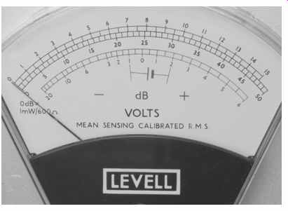
FIG.11 This AC microvoltmeter explicitly states that it responds to the
mean level of (the rectified) AC waveform and is calibrated to give a correct
RMS reading for sine waves only.
Crest factor
A waveform composed mainly of high-amplitude narrow spikes is difficult to measure, so this property is defined.
Crest factor = Vpk / VRMS
Unlike a cheap DVM, a true RMS DVM does not assume a sine wave and apply a conversion factor, instead, it actually calculates VRMS for the waveform from first principles.
Although you and I can calculate VRMS for any waveform, true RMS DVMs are somewhat more limited, and they specify their limitation by stating the maximum crest factor that can be tolerated whilst accurately determining VRMS. As an example, the Fluke 89 IV true RMS DVM can compute RMS accurately provided that the crest factor is <=3 x FSD.
Although DVM manufacturers make a big fuss about true RMS, there is only one time when we really need the facility, and that is when measuring AC heater voltages when the wave form has become distorted and we are truly concerned about the precise heating effect. Otherwise, we can knock true RMS off our shopping list when choosing a good DVM. In practice, if we decide that we want a particularly accurate DVM, we often find that the facility is included whether we want it or not.
Speed of measurement
Despite the prevalence of DVMs, moving coil meters still have their uses. A moving coil multimeter flicks quickly to its reading, and this may warn you to switch off sufficiently quickly to avoid damage.
The industry standard meter in the tube era was the AVO Model 8 moving coil multimeter -- which is still available.
You will find many circuit diagrams stating that voltages were measured using a 20 kOhm/V meter, which refers to the loading that the AVO 8 imposes on the circuit. Unfortunately, the AVO 8 has a heavily damped movement, making it frustratingly slow to use, so the author prefers a really cheap moving coil meter (see FIG.12).
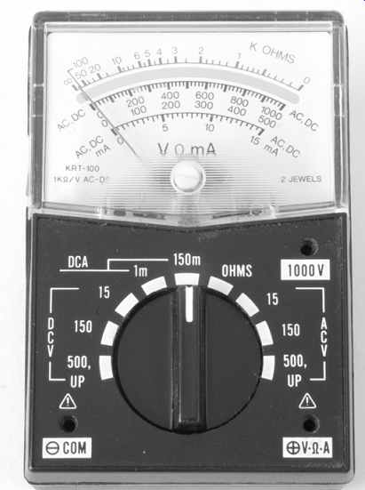
FIG.12 This cheap moving coil multimeter responds quickly, so it is still
useful!
Digital voltmeters (DVMs)
We have mentioned DVMs in passing, but it is now time to consider them in detail. The main advantage of a DVM is that it can be designed to achieve arbitrary accuracy, whereas moving coil meters require precision mechanical engineering (springs, bearings, individual calibration), powerful magnets (with a substantial proportion of expensive cobalt) to achieve an accuracy of +-0.5% at best.
Despite the fact that we don't actually know what time really is, we can measure it stunningly accurately very cheaply. (You would be annoyed if the digital watch given away with a gallon of engine oil had an error of one minute in a week, yet this corresponds to an error of <10 parts per million.) Thus, whenever possible, digital measuring systems convert the measurement of the required parameter into a measurement of time. Unfortunately, if time is used to make the measurement, we must inevitably take time to make that measurement -- usually by counting the pulses of a master clock. Thus, the 0-2V range of a 3 1/2 digit DVM might correspond to counting from 0 to 2000 pulses, and displaying that count scaled by an appropriately positioned decimal point. More significantly, if we wanted a 4 1/2 digit DVM, it would need to count 20 000 pulses, which would either take ten times as long, or require a master clock ten times faster.
We are now in a position to compare DVMs. The natural attitude is to say, ''I want maximum accuracy with minimum cost, and I'm not really bothered about measurement time.'' Expensive experience forces the author to state that you are bothered about measurement time. It is not sufficient for the DVM to make the measurement once and stop, it must make the measurement repeatedly. As an example, we might want to set the anode current in an output stage to precisely 140mA by adjusting a variable resistor. When we adjust the resistor, anode current changes instantaneously, but it takes time for the DVM to make the new measurement that reflects this change, by which time, we may have overshot our adjustment.
Remember that we usually measure to check that a parameter isn't wrong. If it is wrong, we must minimize the time that it is wrong, to minimize the smoke -- so the addition of measurement time to human reaction time might risk the survival of a set of output tubes worth $350. You can buy a very good DVM for $350, yet one measurement might recoup that cost.
Are you still unconcerned about measurement time? A DVM is fundamentally a precision analog to digital convertor (ADC) preceded by switchable attenuators and amplifiers. All ADCs have the following relationship:
cost = sample rate x number of bits
In terms of a DVM, the sample rate is the number of measurements per second, and the number of bits reflects the basic accuracy of the DVM- usually best on the 2V or 5V DC range.
Although DVM manufacturers are open about errors and price, they tend not to mention measurement speed. In an effort to beat the price/performance equation, DVMs often add an '' analog'' bar graph display to their digital display. The bar graph display is not accurate, but it is fast. Because any bar graph display must be composed of discrete segments, it is usually supported by auto-ranging electronics to allow it to display small changes. The upshot is that the display faithfully displays instantaneous changes, but the precise value is unknown.
In short, although bar graphs are very useful for revealing unstable parameters, nothing beats a fast accurate measurement, and this is one of the fundamental differences between cheap and expensive DVMs.
Minor points when choosing a DVM
Some models may not measure current, but this is not a great loss, since to measure current you must break a wire and later reconnect it. Others may measure capacitance, but they are not usually particularly accurate and do not measure small capacitances very well, so you may feel that it is better to put money aside towards a second-hand component bridge.
Some DVMs are the size of an (overgrown) pen, allowing you to read the display without looking away from the position of the probe tip. One very useful feature on a DVM is a resistance range that is guaranteed not to switch diodes on, because this allows you to measure resistors in circuit without semiconductors upsetting the measurement. The better DVMs usually don't have this facility because restricting the applied voltage to 200mV makes it more difficult to achieve a precision measurement. If you are forced to have only one digital multimeter, you need a fast meter that probably includes a bar graph to allow changing values to be clearly seen.
Summarizing, there is no such thing a single perfect meter, and each type has its advantages and disadvantages. Once you start testing, you will quickly discover that you can't have too many meters, so it's worth having different types. At the last count, the author had five DVMs and three analog meters.
Analog oscilloscopes
There is a great deal of software available for converting a computer with a soundcard into a clumsy oscilloscope. Forget it. A 192 kHz soundcard has a maximum theoretical bandwidth of only 96 kHz, and you need far more than that.
The author has not previously recommended oscilloscopes because they were expensive and require skilled use and interpretation, but prices are falling and people are becoming more knowledgeable. However, there is a catch. Analog oscilloscopes use a cathode ray tube (CRT) to produce the display, which requires ~10 kV of EHT to accelerate the electrons to the phosphors. High-voltage circuits are always fragile, and oscilloscope EHT supplies are no exception. Although many parts are generic, the step-up transformer and voltage multiplier chain are invariably specific to the instrument, and may no longer be available. If you buy a cheap second-hand 20MHz oscilloscope, and it fails after a few years, it will probably have paid for itself, but second-hand >100MHz oscilloscopes are more expensive, so an irreparable failure is galling.
Whether you are using the latest technological confection from Tektronix, complete with all possible bells and whistles, or a 5MHz dinosaur from a junk shop, the principles are the same.
An oscilloscope is simply an electronic graph drawing machine that draws graphs of voltage (vertical, or ''Y'' axis) against time (horizontal, or ''X'' axis).
An analog oscilloscope uses a CRT to draw the graph by repeatedly tracing a beam of electrons onto the fluorescent phosphor screen to form a visible trace. The CRT is a large tube with focusing anodes (collectively known as an electron lens) that shape the electron stream from cathode to final anode into a beam that is brought into focus on the fluorescent phosphor coating on the inside of the tube face to form a sharply defined spot. The phosphor coating is not conductive, but current flows because the electrons in the beam strike the phosphor so hard that one fast-striking electron releases a slow-moving secondary electron in addition to a photon of light. The slow-moving electron is easily attracted to the concentric final anode, and thus a circuit is formed. The spot is scanned repeatedly across the tube face by applying a ramp waveform to the horizontal deflection anodes, and the persistence of the phosphor coating coupled to the persistence of the eye produces a continuous display.
In order to produce a stationary trace, all oscilloscopes have three main blocks which have to be adjusted correctly (see FIG.13).
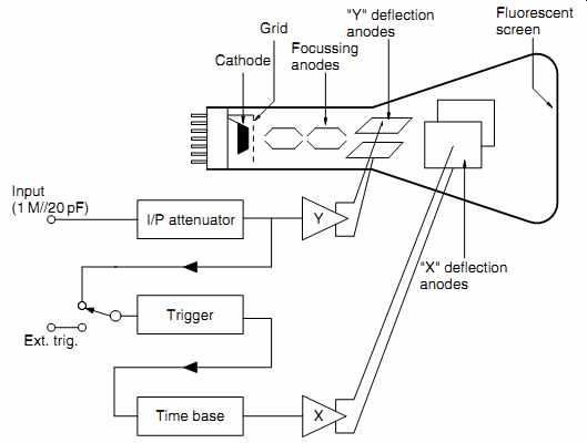
FIG.13 Analog oscilloscope block diagram
The ''Y'' amplifier
The ''Y'' amplifier is responsible for controlling the deflection and positioning of the beam in the vertical direction of the display tube. Adjustment of the relative DC potentials on the ''Y'' deflection anodes shifts the beam. Adjustment of the input attenuator controls the sensitivity of the deflection - commonly labeled in volts/div. This control uses a 1, 2, 5 sequence because it gives equal spacing on a logarithmic graph and allows the oscilloscope to adapt smoothly to the natural world. (Currency uses this logarithmic sequence for the same reason)
There is often a fine control (sometimes called variable, or vernier) that allows the vertical scaling to be finely adjusted to make the waveform conveniently fit on the screen. You can't measure the voltage anymore, but most of the time, we use an oscilloscope because we are more concerned about the shape of the waveform.
All oscilloscopes also have a choice of input coupling, marked AC, DC, or GND (see FIG.14).
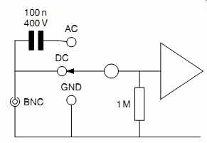
FIG.14 Input coupling to the ''Y'' amplifier
-- DC: All signals, including DC, are passed to the deflection anodes. This is the preferred mode of operation as it does not attenuate low-frequency signals, and therefore does not distort square waves, but it may not be practical when investigating small audio signals in a tube circuit.
-- AC: DC is blocked by a capacitor, this is useful for investigating the AC conditions of a circuit separately from the DC conditions - such as faultfinding.
-- GND: This connects the input of the oscilloscope to ground/ ground. If the trace is then moved to a convenient reference point, when returned to DC coupling, the movement of the trace from the reference allows the applied DC to be measured easily. (Using an oscilloscope to measure DC might seem like a sledgehammer to crack a nut, but it responds faster than even an analog meter, so it can be very useful when faultfinding.)
The time base and “X” amplifier
The time base provides the horizontal, or “X”, sweep, in a 1, 2, 5 sequence typically ranging from milliseconds per division to nanoseconds per division. As with the “Y” amplifier, there is often a variable control that finely adjusts the horizontal scaling to make the waveform conveniently fit on the screen, but the horizontal sweep is now uncalibrated, so absolute time measurements can no longer be made.
The time base control adjusts the frequency of a precision ramp generator. Because the oscilloscope display tube uses electrostatic deflection anodes to deflect the beam by an amount proportional to applied voltage, the combination of the two produces a sweep where horizontal deflection is proportional to time.
Depending on the tube type and final EHT voltage (higher HT makes the electrons travel faster, making them more difficult to deflect), the deflection anodes require ~200V[pk-pk] to deflect the beam from one side of the tube face to the other. A dedicated high-voltage “X” amplifier very similar to the “Y” amplifier is therefore required to deliver the sweep voltages required by the tube.
If the sensitivity at the input of the “X” amplifier is made the same as that at the input of the “Y” amplifier, the “X” amplifier's input can be switched to accept either the ramp from the time base generator, or Ch2 (leaving Ch1 to go to the “Y” amplifier). This is known as “XY” mode, and because it is so cheap to provide, all oscilloscopes offer it. “XY” mode allows the display of Lissajous figures -- these are virtually useless, but are loved by producers of science fiction programs and “James Bond” films (see FIG.15).
The Lissajous figure in the diagram compares the voltage waveform across a choke with the current waveform through it. Because the phase between current and voltage is zero at resonance, and changes very sharply around it, testing for phase is a very sensitive way of determining resonant frequency. When the two waveforms are in phase, a perfect straight line results, rather than an ellipse.
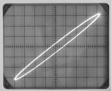
FIG.15 A Lissajous figure showing a perfectly straight line (rather than
a slight ellipse) would indicate zero phase error.
Triggering
If we were to allow the time base to sweep randomly with respect to the input signal, we would see a mess of moving patterns on the screen. We need to sweep the electron beam in such a way that it draws each trace perfectly overlaid onto the previous trace, thus producing a single trace of the input wave form. If instead of letting the time base sweep continuously, we only allowed it to begin a sweep at the instant that a particular feature of the input waveform had been identified, this would synchronies the time base to the input signal and force the traces to overlay.
The trigger identifies the significant part of the input signal's waveform both by its absolute level and whether that voltage is rising or falling.
The simplest form of triggering is AC, which triggers the time base each time the input waveform passes through zero. DC or normal triggering allows the trigger voltage to be determined by the user adjusting the trigger level control. Whether in AC or DC mode, trigger slope can be chosen to be + (rising edge) or - (falling edge) (see FIG.16).
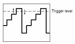
FIG.16 The trigger identifies a unique point on the waveform using a
combination of voltage and slope
In this example, the trigger level has been set so that the oscilloscope trigger fires on the top step of the staircase wave form. But the waveform goes up the step, then down, so if the trigger fired on both edges, we would see two traces, one shifted horizontally from the other. To avoid this problem, trigger slope enables us to select whether the trigger fires on the rising or falling edge.
Note that most analog oscilloscopes produce a sweep that is slightly wider than the display, so the start of the sweep at the trigger point and the end of the sweep are not seen unless deliberately shifted onto the screen.
Because in this example the time base has been set to show more than one cycle of the waveform, the oscilloscope would only manage to sweep half way across the screen before being triggered again, starting a new sweep, so it would never manage to sweep all the way across the screen. To prevent the problem of truncated sweeps, once the trigger has fired, it is guarded until the time base has completed the sweep and is ready to begin the next.
If the time base is only allowed to sweep after the trigger has been fired, it is known as normal triggering. However, the disadvantage of normal triggering is that if you haven't been able to trigger the oscilloscope, you don't have a display, so you don't know why you have failed to trigger. To circumvent this problem, oscilloscopes have AC auto triggering (occasion ally known as bright line) which automatically triggers the time base after each sweep (free run), or is triggered when the trigger waveform passes through 0V. Although this mode of triggering can cause an unlocked trace, it makes it easier to determine which controls need to be adjusted to produce the required display.
The signal may contain noise that we want the trigger to ignore.
If we were looking at a small signal in a pre-amplifier, it might well have high-frequency noise on it, and if we were to allow that noise to reach the trigger, it would make the display of our wanted signal unstable. (Remember that noise is proportional to the square root of bandwidth, so a 20MHz oscilloscope sees 30 dB more noise than we can hear in the 20 kHz audio band width.) For this reason, manufacturers include HF reject, which is typically a ~30 kHz low-pass filter at the input to the trigger. Conversely, our small signal might be riding on some mains hum, and we might be able to reject this using LF reject (high-pass filter at ~80 kHz), but we will see a much better way in a moment.
The trigger needs to be provided with an input signal from which to trigger. Internal triggering picks off one of the signal channels after their attenuators, and is typically marked Ch1 or Ch2. External triggering may come from a front panel BNC or from AC line, which is the mains supply.
Suppose that you are investigating an amplifier, and have applied a 1 kHz sine wave from an oscillator to its input, by definition, signal levels within the amplifier change as you move from test point to test point, probably requiring adjustment of trigger level if internal trigger is selected. However, if you also connect the oscillator to the external trigger input, and trigger from this point, the display will always be correctly triggered, no matter where you probe, and no matter how much noise or equalization has been added to your signal.
External triggering is almost always better than internal, so it is a good idea to get into the habit of using it.
Similarly, when you are investigating mains hum, if you select AC line, the trace will always be locked. Incidentally, if you suspect that you are seeing mains hum, but are not sure, if the trace becomes stationary when you flick the trigger to AC line, mains hum is confirmed.