Bandwidth
The most important single specification for a motorcycle is its engine capacity and the counterpart for an analog oscilloscope is bandwidth. And just like the motorcycle, an oscilloscope's bandwidth is invariably prominently displayed next to its maker's name.
Strictly, bandwidth is defined as the difference in frequency between the HF and LF roll-offs where the response has fallen by 3 dB. Thus, an FM tuner might define the bandwidth of its 10.7MHz intermediate frequency amplifier as being 10.85MHz - 10.55MHz=300 kHz. Because all oscilloscopes respond to DC (which is 0Hz), it is sufficient to specify an oscilloscope's bandwidth simply by quoting the HF roll-off.
A 20MHz oscilloscope is probably the slowest new oscilloscope that you could buy today, and this is just fast enough for audio. But if the ear can only hear to 20 kHz, why do we need one thousand times as much bandwidth? The first clue is in the definition of bandwidth. A 20MHz oscilloscope will display a 20MHz sine wave, not at its correct amplitude, but attenuated by 3 dB. A well-focused trace is just capable of displaying a 1% amplitude error, so we would ideally like the limited bandwidth of our oscilloscope to contribute a smaller error, perhaps 1/2% error, at the highest frequency for which we want to be able to measure amplitude correctly. If the oscilloscope's transient response has been optimized, its HF response corresponds to that of a single CR network, and we find that for 1/2% error we need the -3 dB frequency to be ten times higher. In other words, our 20MHz oscilloscope introduces its own amplitude errors above 2MHz. (It is precisely this 10:1 ratio that justified the existence of 60MHz oscilloscopes - traditional analog television signals had a bandwidth of 5.5MHz.) Having established that our 20MHz oscilloscope is only accurate to 2MHz, this is still way beyond 20 kHz, so why do we need this bandwidth? Unfortunately, prototype audio power amplifiers do not always behave as they should, and it is not uncommon to find them oscillating between 1 and 2MHz, so our oscilloscope needs to be able to display any oscillation perfectly in order that we can see it, and do something about it. There's an old saying that you can be neither too rich nor too thin. As far as oscilloscopes are concerned, you can't have too much bandwidth.
The other parameter that goes hand in hand with bandwidth is the fastest time base speed. The ideal display contains one or two cycles of the waveform. Taking 20MHz as an example, the period (duration of one cycle) is:
T = 1/f = 1/[20 x 10^6] = 50 ns
Oscilloscope screens generally have ten horizontal divisions, so to display two cycles of 20MHz, we need a time base that sweeps five divisions in 50 ns. In other words, it needs to be able to sweep at 10 ns/div. In practice, very few 20MHz oscilloscopes are able to sweep as fast as this, and the author's (cheap and cheerful) Gould OS245A fastest sweep is 1 ms/div, so it can only adequately display 200 kHz, despite being described as a 10MHz oscilloscope. This isn't really fast enough for faultfinding audio, because the easiest route to curing unwanted oscillations is to find a circuit change that alters the frequency of oscillation. Once that has been done, curing the oscillation is usually easy.
For faultfinding power amplifiers, we would ideally like a time base that can sweep at 100 ns/div, or better. The next step up from 20MHz is a 100MHz oscilloscope such as the 1970s vintage Tektronix 465, which can sweep at 20 ns/div and has lots of extra features which we now need to investigate.
Bells and whistles
Bells and whistles allow detailed examination of more complex signals, but these refinements still fall into the basic three blocks of “Y” amplifier, time base, and trigger.
The “Y” amplifier
Frequently, we need to investigate more than one signal at a time and compare relative timings or voltages. To do this, we add extra input attenuators and amplifiers, and switch sequentially between them at the input to the final “Y” deflection amplifier (see FIG.17).
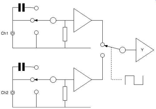
FIG.17 Adding channels to an oscilloscope simply requires additional
attenuators, input amplifiers, and an electronic switch.
Older oscilloscopes require you to choose between alternate or chop modes to switch between the channels. As the names suggest, alternate mode sweeps alternately between Ch1 and Ch2, and this is best for time base settings >2ms/div, but below that, chop mode is better because chopping between the channels as they are swept avoids flicker at slow time base speeds.
Although most oscilloscopes have two channels, some modern oscilloscopes can display up to four input channels at once, but the screen becomes rather cluttered, and the display dims.
(Brightness at a given point is proportional to the number of electrons striking that point, so if the electron beam has to produce four traces instead of one, each trace must be reduced to one quarter of the brightness of a single trace.) Surprisingly, the more significant limitation is that four channel oscilloscopes often do not have a separate triggering channel, so the fourth channel ends up being used as the external trigger, and your extra money actually bought a three-channel oscilloscope (possibly with limited ''Y'' attenuators on Ch3 and Ch4), so check this very carefully.
Cursors are internally generated vertical or horizontal move able lines that are added at the input to the “Y” amplifier and are the modern development of crystal calibrator pips that were sometimes included in early oscilloscopes and radar. Because cursors are digitally generated, the count that produces their position can be displayed as a number, and this number can be modified automatically by “Y” amplifier setting or time base setting to give a read-out directly in terms of time or voltage.
Cursors have three valuable advantages:
-- Without cursors, you measure voltage (or time) by counting squares and multiplying by the volts or time per division -- which is tedious and prone to error.
-- Because the phosphor trace is behind the (thick) glass face of the CRT and the ruled graticule (scale) is on the outside, the absolute position of your eye changes their relative position.
On superior oscilloscopes this parallax error was eliminated by painting the graticule lines on the inside of the CRT face (internal graticule).
-- Measurement referred to a ruled scale assumes that CRT deflection is linear, that deflection amplifiers are linear, and that the time base ramp is linear. In practice, none are perfectly linear, but cursor position is distorted by the same amount as the waveform's features, so all the errors cancel.
The addition of cursors converts the oscilloscope from being a display device into a measuring instrument (see FIG.18).
The time base
Although we argued earlier that we want as fast a time base as possible, a fast time base is rather like looking through a telescope - you can see in great detail, but you don't know where you are looking. High-powered astronomical telescopes solve the problem by fitting a low-power sighting telescope along the barrel of the main instrument. Once the sighting telescope has located the region to be explored, the observer switches to the main instrument. Similarly, fast oscilloscopes use their main or “A” time base to find the region on the waveform to be investigated, then the delayed or “B” time base is engaged to give the detailed view. Since position across a sweep is time, adjusting the delay before the “B” time base fires determines which part of the waveform is to be investigated in detail (see FIG.19).
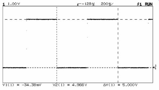
FIG.18 Cursors enable quick and accurate measurement of voltage or time
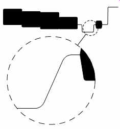
FIG.19 Delayed time base enables detailed examination of any part of
this complex waveform
To help the user, typical oscilloscopes have two intermediate modes between the ''A'' and ''B'' time bases. Intensified mode adds a bright-up to the main display which highlights where the ''B'' time base will sweep. Once the correct region has been chosen by adjusting delay, mixed mode can be engaged, which alternates between ''A'' time base and ''B'' time base, allowing fine delay adjustment with confidence. Finally, the ''A'' display can be switched off by selecting ''B'' time base only, resulting in an uncluttered display of the precise area of interest.
Delayed time base is intended for investigating high-frequency detail buried in a low-frequency waveform, so it is particularly suitable for investigating:
-- Ringing in HT supplies caused by diode switching
-- Ringing at the leading edge of square waves caused by incorrectly terminated audio transformers
-- Heater noise spikes caused by diode switching.
Using the delayed time base tends to dim the display, so the fastest oscilloscopes use CRT image intensifier techniques (as used in night sights) to make the display brighter, but at increased cost.
Triggering
In order to use the improved time base system effectively, the triggering must become more sophisticated. Early delayed time base oscilloscopes offered a separate trigger for the ''B'' time base, but this isn't particularly useful, so most modern oscilloscopes simply start the ''B'' time base immediately after the delay. (This must be one of the few whistles that has been discarded!) Other features include triggering on numbered television lines or pattern triggering where the trigger recognizes a pattern such as a particular sequence of logic pulses.
Holdoff is a very useful facility that allows the trigger to be guarded by an adjustable time, so that only the intended transition triggers the oscilloscope. This facility is particularly useful for persuading an oscilloscope to synchronies to the data words in the serial digital data stream leaving the S/PDIF output of a CD player.
Digital oscilloscopes
Analog oscilloscopes apply an amplified input waveform directly to the CRT, so it must have the same bandwidth as the ''Y'' amplifiers. 20MHz CRTs are easily and cheaply made, and even 100MHz is not too much of a problem, but >400MHz is much more expensive, so the 1GHz Tektronix 7104 was a very rare beast.
Digital oscilloscopes solve the CRT bandwidth problem by divorcing the wide bandwidth of the input waveform from the display. They do this by converting the analog waveform into digits, storing them in memory, and reading them out at a (much slower) rate chosen to suit the display. Thus, when digital oscilloscope manufacturers refer to bandwidth, they mean the analog bandwidth of the attenuator and input amplifier system up to the input of the ADC. Not only does storing and displaying the waveform at a slower rate mean that an extremely cheap display is perfectly suitable for a 5GHz oscilloscope, but it also means that a faster time base is easily achieved. As an example, the (now obsolete) 100MHz HP54600B can sweep at the ideal 2 ns/div, enabling two cycles of 100MHz to fill the screen.
Because digital oscilloscopes are so much cheaper to make, the major manufacturers no longer offer analog oscilloscopes.
Nevertheless, despite all the fuss made by marketing departments, a good analog oscilloscope such as the 1970s vintage 350MHz Tektronix 485 takes a lot of beating. To make an informed choice between buying a new digital or an old analog oscilloscope, we will need to investigate some of the murkier areas of digital principles about which some oscilloscope manufacturers are distinctly coy.
The ADC ( Analog to Digital Convertor)
Only digital oscilloscopes have an ADC, commonly known as the acquire block, and its principles of operation need to be understood to obtain good results.
Sampling and quantizing
An analog signal can change continuously in both time and voltage. Digital oscilloscopes take the analog signal and break it up in time (sampling) and in voltage (quantizing).
Having broken the signal, they convert it to a stream of binary digital numbers that describe that signal.
When an analog signal is quantized, there are always errors because the analog voltage cannot be perfectly described by a finite number of quantizing levels (see FIG.20).
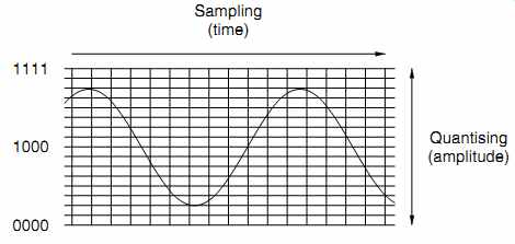
FIG.20 Quantizing breaks voltage into steps; sampling breaks time into
steps. The two operations are separate and can be applied in either order.
As an example, the 100MHz Tektronix TDS3012 has 29 (512) quantizing levels, which means that if a voltage falls between two levels, there will be a maximum error of +-0.1%. Given that +-0.1% quantization error is trivial compared to the +-2% analog errors in the input attenuator and amplifier section, you might feel that using nine bits is extravagant in terms of ADC and memory cost. There are two justifications for this bit depth:
-- 512 quantizing levels map ideally (with a small overlap) onto a standard LCD screen having 480 vertical pixels, so this is a worthwhile advantage.
-- Because the quantizing errors are so small, a trace can be expanded by a factor of ten after capture, allowing investigation of details without quantizing errors becoming too noticeable.
We have seen that quantization (voltage) errors are almost insignificant. Unfortunately, sampling (time) errors are far more of a problem.
Nyquist and equivalent sample rate
The Nyquist criterion states that the original waveform can be correctly reconstructed provided that the sampling frequency is at least double the highest frequency to be sampled. Practical considerations increase this frequency slightly, so CD uses 44.1 kHz sampling frequency even though its audio bandwidth is limited to 20 kHz. This simple theory implies that a 100MHz oscilloscope requires an ADC that samples at 200MS/s (megasamples per second), yet the HP54600B can only sample at 20MS/s, whereas the TDS3012 can sample at 1.25GS/s.
Why do these two 100MHz oscilloscopes have such wildly different sample rates? Equivalent sample rate.
The HP uses a technique known as equivalent sample rate (called repetitive sample rate by LeCroy), and it works like this:
We assume that the input signal is repetitive, perhaps a 100MHz sine wave. Sampling at 20MS/s means that we sample at 50 ns intervals, but an entire cycle of 100MHz only lasts for 10 ns, so we miss four entire cycles completely and sample a single point on the fifth cycle. This doesn't sound very useful, but if we were to delay sampling after the next trigger point by a time equivalent to one hundredth of the screen width, our next sample would be at a slightly later point on the waveform, and would therefore plot a different voltage. If we keep on incrementing the sampling time delay after trigger by one-hundredth screen width intervals, we eventually build up an entire waveform that appears to have been sampled at a much higher rate. Thus, if we had set our time base to 2 ns/div (to display two cycles of 100MHz), the sweep would display 20 ns, and if we had set our delay increments to give one hundred points, we would appear to be sampling every 0.2 ns, giving an equivalent sample rate of 5GS/s. Very clever, yes? The problem with equivalent sample rate is in the assumption that the input waveform is repetitive. A general rule of thumb for oscilloscopes is that you need at least ten points in a cycle to give a reasonable approximation to the shape of that wave form. But if your waveform is a one-off pulse, the ADC needs to take a genuine ten samples in one cycle, so a sample rate of 1GS/s is needed to give a reasonable approximation of a 100MHz sine wave in one-shot mode. Thus, the TDS3012 does have a one-shot bandwidth of 100MHz, but the 20MS/s sample rate of the (much earlier) HP54600B means that it has a one-shot bandwidth of only 2MHz.
Contravening Nyquist and aliasing
If we apply a frequency ( fm) that is higher than half the sample frequency ( fs) to an ADC, the frequency of the input signal will be misinterpreted as a low frequency, and this phenomenon is known as aliasing (see FIG.21).
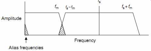
FIG.21 Once fm > fs - fm, alias frequencies begin to crawl up from
0Hz
When digital audio is recorded, the ADC is preceded by a low pass anti-aliasing filter set to slightly less than half the sampling frequency. In this way, aliasing is eliminated, but as we will see in a moment, digital oscilloscopes cannot incorporate an anti aliasing filter, so they are susceptible to this problem.
Sample rate, record length, and time base speed
Remember that a digital oscilloscope samples the incoming signal and writes the results into memory. Later, the memory is read to the display at a convenient rate. Suppose that we want to display two cycles of 100MHz, and we have chosen an ADC that can run at 1GS/s. Each cycle generates ten points and we have two of them, so we generate twenty points across the screen. Now suppose that we want to display two cycles of 50Hz. Each cycle lasts 20ms, so the total sweep lasts for 40ms.
In that time, sampling at 1GS/s, we generate 40 000 000 points, requiring a lot of memory. Worse, we write to that memory at 1GHz. Unlike computer memory, we don't need to be able to access data points in this memory in a totally random fashion, so there are various fudges, collectively known as demultiplexing, that allow the use of slower memory. Nevertheless, oscilloscope memory is expensive, and in 2003, upgrading a LeCroy 8600A 6GHz 10GS/s 4ch oscilloscope from its standard 2Mpt memory to 50Mpt increased the price of the oscilloscope by 57%.
We ideally need an entire screen of memory either side of the screen, which would enable a feature at one extreme side of the screen to be moved to the other extreme without bringing a blank space onto the screen. In addition, it would be nice to have enough samples in memory to allow the trace to be expanded without generating visible gaps on the display. If we had 10 000 samples allocated across the screen, a basic computer display 640 pixels wide would allow us to expand by a factor of ten without producing visible gaps. To allow a screen either side, we would need to store a total record length of 30 000 samples, of which 10 000 would occupy the screen at any one time (see FIG.22).
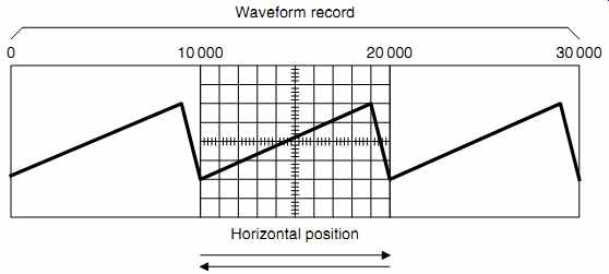
FIG.22 The horizontal position control moves the display window back
and forth across the waveform record
The screen has ten divisions, so we can find the maximum permissible sample rate using:
Maximum permissible / sample rate = visible record length / 10x time/div
Note that sample rate is now totally dependent on the amount of memory, so if we set the time base to 10 ms/div, our example oscilloscope having a visible record length of 10 000 points would be forced to drop its sample rate from 1GS/s to 100MS/s. This isn't a problem, because even if we required ten points per cycle, this sample rate and time base setting could correctly capture one thousand cycles at 10MHz, and we would never be able to distinguish this number of cycles across the screen, so the display would be identical to an analog oscilloscope. In practice, the argument is complicated by the fact that we only display 640 of the 10 000 points in memory, but because we have correct data in memory, tricks can be applied to greatly reduce the inevitable aliasing caused by the re-sampling needed to accommodate the display.
It might seem odd to choose 10 000 points across the screen when we know that we will have to re-sample to 640 pixels, but 10 000 produces nice round numbers for the sample rates generated by the 1, 2, 5 sequence of the time base.
Because sample rate varies with time base setting, we cannot precede the ADC with an anti-alias filter, and this means that aliasing is always a possibility. As an example, analog video contains high and low frequencies simultaneously, and an oscilloscope set to 10 ms/div will display almost two television lines which contain significant energy at 4.43MHz (3.58MHz USA), and although the TDS3012 can display this with insignificant aliasing, the short record length of the HP54600B causes sufficient aliasing to render the display almost unusable.
Summarizing; at slow time base speeds, it is record length that determines sample rate and you can't have too much memory.
Be warned that because oscilloscopes access their memory at such high speeds, their data busses are transmission lines and extra memory cannot simply be added in the manner of a PC, so the choice has to be right at the moment of purchase.
Features unique to digital oscilloscopes
We have found that a high sample rate is crucial, but that it can only be maintained at slow sweep speeds by having sufficient record length, and that analog bandwidth becomes a secondary consideration. Worse, because digital oscilloscopes are really computers with knobs on, they obey Moore's law (speed doubles every 18 months), and depreciate almost as fast as a PC, so any oscilloscope with a maximum sample rate of less than 100MS/s (appropriate for 20MHz analog bandwidth) is effectively junk. Despite these caveats, digital oscilloscopes have many features that simply cannot be provided in an analog oscilloscope, so it is time to look at their advantages.
Negative time
Because digital oscilloscopes acquire, store, and display the input signal continuously, they can show events before the trigger point, allowing them to look backwards in time. By definition, this is impossible for an analog oscilloscope.
Usable slow time base settings
At very slow sweep speeds, an analog CRT no longer produces a graph, but a decaying swept spot, making the display very difficult to interpret. At these slow sweep speeds, digital oscilloscopes stop triggering, and free-run (known as roll mode), which produces a non-decaying display akin to an analog chart recorder, allowing sweep speeds of 10 s/div, which is very useful for observing events like heater warm-up times.
Capturing and displaying infrequent events
An analog oscilloscope produces trace brightness proportional to the time spent by the beam sweeping overlaid traces per second. If the oscilloscope spends most of its time waiting to sweep, the trace dims. By contrast, even a single trace written into digital memory can be written to the display repetitively to give a bright trace.
Color
The color of the trace on an analog oscilloscope is deter mined by the required persistence of the phosphor screen coating, so the trace produced by Ch1 is the same color as that produced by Ch2. Digital oscilloscopes can use television type displays (CRT or LCD), allowing the two traces to be different colors, which means that instead of using the top half of the screen for Ch1 and the lower for Ch2, both traces can occupy the full height of the screen because they are easily identified.
The previous point is more important than at first appears. The screen's ''Y'' axis corresponds directly to the codes ranging from 0 to 512 (9 bit ADC) leaving the ADC. If we only use half the screen for one channel (0 to 256), we have effectively thrown away one bit of ADC resolution, so we must always use the full height of the screen to maximize accuracy. Of course, the same argument could be leveled at an analog oscilloscope, but the significance is that reduced trace height degrades the accuracy of automated measurements. If we have two waveforms occupying the full height of the screen, they can only be easily distinguished if they are of different colors, so for a multi-channel digital oscilloscope, a color display is a necessity rather than a luxury.
Storing and exporting traces
The digital advantages mentioned previously pale into insignificance compared with the ability to store traces for later comparison. When fettling an amplifier and testing the effect of changing a component, it is extremely useful to be able to compare ''before'' and ''after''. Most digital oscilloscopes can export traces, but some require an add-on module, plus proprietary software on the PC, and perhaps a specific card in the PC. This all costs money, and data transfer requires the oscilloscope to be connected to the PC, which is a nuisance.
The ideal oscilloscope has a 3.5" floppy drive using PC formatted diskettes so that you can simply store a trace and take the diskette to any PC at your leisure. This requirement greatly reduces the value of older digital oscilloscopes, so if you are considering buying one, check very carefully how it exports traces.
A very powerful oscilloscope may encounter a somewhat different problem in that it has such a large record length that its trace files are simply too large to fit on a floppy disk. These oscilloscopes must transfer their data via a network port. At the time of writing, amateurs are unlikely to encounter this problem because such oscilloscopes are still quite expensive, but prices are falling all the time.
Peak detect/data compaction and glitch detection
At slow time base speeds, finite record length forces the oscilloscope to lower the rate at which it writes to memory, so it may miss an important event (perhaps a glitch) that occurs between samples. Peak detect mode captures such transients by running the ADC at its maximum sample rate, but only records the highest (or lowest) voltage and drops this result into the nearest available memory location (see FIG.23).
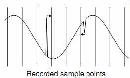
FIG.23 When sample rate falls, a fast event can fall between recorded
samples, so peak detect detects such events and records them at the nearest
memory location.
The fact that such events are recorded with a slight time error and gross distortion is not nearly as serious as missing the event altogether. Peak detect alerts the user that a more detailed investigation is necessary and is invaluable for finding the cause of otherwise insoluble faults, such as those caused by random spikes on the output of a faulty switched mode power supply.
A slightly more sophisticated alternative called data compaction by LeCroy is to measure the highest and lowest voltage, and record both at the nearest available memory location. Since two items of data are recorded, rather than one, this approach immediately doubles the amount of memory required for a specified record length.
Averaging and noise
Because a digital oscilloscope effectively stores the data resulting from each sweep as a database, it can perform mathematical calculations such as averaging. The oscilloscope displays a repetitive waveform, so each sweep across the screen draws a trace identical to the one before it. If we average across traces, the repetitive element stays the same, but any random noise on the traces averages to zero. Averaging is a very powerful method of extracting signals seemingly buried in noise. Typically, averaging can be adjusted in binary logarithmic steps (2, 4, 8, etc.) from 2 to 512 traces. The reduction in noise is proportional to ??? n p so averaging over 512 traces reduces noise by 27 dB, but at the expense of drastically slowing the time taken for the display to stabilize. If the oscilloscope is triggered from the source of cross talk, averaging is very useful for detecting crosstalk from one channel into the power supply or to another audio channel.
Envelope
Envelope mode never deletes a sweep, so successive sweeps are displayed over one another in the manner of a multiple exposure photograph. Although the display may become completely distorted, making it impossible to discern a recognizable wave form, it enables maximum voltage excursions to be measured easily, and this is particularly useful for determining how much overload capability is required in a given stage. We simply apply music for as long as we like and measure the maximum vertical excursion. Conversely, data communications engineers use envelope for measuring time jitter (horizontal excursion) on their data waveforms.
Displaying a sweep indefinitely is not always ideal, so envelope mode is often adjustable in 2, 4, 8 steps to limit the number of sweeps for which the results of a given sweep are stored and displayed, and this enables the appearance or disappearance of infrequent pulses to be monitored.
Adjustable persistence
All displays (and the human eye) have a property known as persistence, whereby a gradually decaying visible image remains even though its cause has gone. This might seem to be a defect, but it can be quite useful because it assists in seeing momentary events. Persistence in an analog oscilloscope is pre-determined by the choice of display phosphors and is unchangeable.
Now that memory has fallen in price, digital oscilloscopes can mimic persistence electronically and controllably. The way that this is done is to treat the array of display pixels as a 3D database.
Early digital oscilloscopes simply placed a ''1'' or a ''0'' in each pixel on each trace. This meant that infrequent events were displayed with exactly the same brightness as frequent events, leading to a confusingly cluttered display. However, if a 4-bit number is stored at each pixel, it can be incremented by one each time the waveform hits that pixel (perhaps from 0100 to 0101). If a calculation is applied simultaneously that gently decrements that number over time, pixel brightness can be made proportional to that number, and we have recovered the analog advantage of persistence. The technique is known as digital phosphors and allows a digital oscilloscope with sufficient sample rate to produce a display almost indistinguishable from a top quality analog oscilloscope, but with all the digital advantages.
This truly is the best of both worlds, and was the deciding factor in the author's purchase of a TDS3032.
The key difference between persistence and envelope is that envelope switches pixels off abruptly whereas persistence exponentially reduces the brightness of older pixels (see FIG.24).
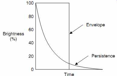
FIG.24 Persistence (exponential decay) versus envelope (abrupt switch
off) brightness
Dots and vectors
Because the oscilloscope samples and quantizes, it plots dots on a screen of graph paper. It is conventional to join the dots on graph paper, and oscilloscopes can also perform this function. Some oscilloscopes offer the user a choice of the way in which the journey is made (straight line, or sin(x)/x curve) from one point to the next; so this feature is usually known as vectors. However, there is an implicit assumption in joining the dots that the curve really did move smoothly from one dot to the next. Finite sample rate means that this assumption may not be true, particularly at slow time bases, so most oscilloscopes can be switched to dots only.
Automated measurements
A display on an oscilloscope is likely to contain one or two cycles of a waveform. Each cycle is thus a histogram composed of many vertical bars, and measurements or calculations that involve maxima, minima, or areas under one cycle of the graph can easily be made. Provided that the oscilloscope can display the waveform without distortion, a digital oscilloscope can calculate VRMS or Vmean, etc. for any waveform, and accuracy is limited only by the number of samples taken per cycle and the number of quantizing bits used. Normally, as many cycles as are available in the wave form record are used for calculation, but cycle RMS and cycle mean are found by considering only the first cycle after the trigger.
The great advantage of automated measurements is that they are live and update as the waveform changes.
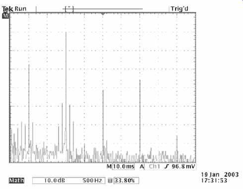
FIG.25 This FFT shows the amplitudes of the 2nd to 6th harmonics of a
push-pull output stage. As expected, the odd harmonics are higher amplitude
than even, but more interestingly, there are 50Hz spikes around the 2nd and
3rd harmonics caused by intermodulation with a poor power supply
Fast Fourier Transform (FFT)
The FFT is a mathematical tool that allows data captured in the time domain to be displayed in the frequency domain. Put simply, although the vertical axis is still voltage, it is now plotted against frequency, rather than time, and the oscilloscope has been converted into a spectrum analyzer. This is an extremely useful facility for investigating distortion harmonics (see FIG.25).
The FFT is an immensely powerful tool, but it has limitations.
In converting from time to the frequency domain, the mathematics of the FFT make the assumption that the waveform to be analyzed repeats itself periodically. This assumption may seem trivial, but has major repercussions.
If we captured a single cycle of the waveform, and drew it around a circular drum (like a seismograph) so that the end of the cycle just met the beginning, then by rotating the drum we could replay the waveform ad finitum and reproduce our original signal. Unfortunately, any uncertainty as to the precise timing of the end of the cycle causes a step in level when we attempt to loop the recorded cycle back to itself on replay. However, if we capture more cycles on our drum, this glitch occurs proportionately less frequently and causes less of an error. Thus, capturing a thousand cycles reduces the error by a factor of a thousand, at the cost of needing one thousand times the record length, making an oscilloscope's record length even more important if FFT is to be contemplated.
The other way of reducing the glitch is to force periodicity by applying a window to the waveform record. In this context, a window is a variable weighting factor that multiplies the values of the samples at the ends of the waveform record by zero, but applies a greater weighting (<=1) to samples towards the middle.
Since any number multiplied by zero is zero this forces the end samples to zero, and allows the waveform record to be repeated without glitches (see FIG.26).
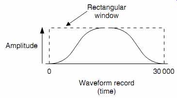
FIG.26 Shaping the window reduces the effects of periodicity violation
compared to a rectangular window
Because windowing distorts the waveform record, it must distort the results of the FFT calculated from that record.
Windowing either spills energy from high-amplitude bins into adjacent bins, producing skirts around frequencies having high amplitude, or it changes bin amplitudes. (Because the process of sampling broke time into discrete slices, the results of an FFT must produce frequencies in discrete slices, and these are known as bins.) All windows are therefore a compromise between frequency and amplitude resolution.
A window that does not modify sample values is known as a rectangular window (because it multiplies by a constant value of 1 over the entire waveform record). Because the rectangular window does not modify sample values, it does not cause spreading between bins, and it offers the best frequency resolution. Unfortunately, amplitudes are likely to be in error because of periodicity violation. Conversely, the Blackman Harris window modifies the ends of the waveform record to avoid periodicity violation, which causes spreading between bins, but improves amplitude resolution. In the same way that averaging reduced noise on a displayed waveform, aver aging can significantly improve the signal to noise of an FFT display, but with the same cost of reduced measurement speed.
Connecting to the oscilloscope
Having acquired our oscilloscope, we need a means of connecting it to the circuit we want to test.
Input capacitance and voltage dividing probes
The most sensitive setting on a typical oscilloscope is 2mV/div and the standard input resistance is 1 M-ohm. This is almost sensitive enough for a microphone, so we must use a screened lead to avoid picking up hum from all the (nearby) mains wiring. Typical coaxial screened lead has a capacitance of ~100 pF/m; perhaps we have bought a 20MHz oscilloscope, and use a 1m lead having 100 pF of capacitance to connect the input of the oscilloscope to the output of a common cathode gain stage using a high m triode such as an ECC83 or 6SL7. Under typical operating conditions, this stage is likely to have an output resistance of 60 kOhm. Unfortunately, the capacitance of the lead and output resistance of the amplifier forms a low-pass filter having a -3 dB frequency of:
f = 26.5kHz

We cannot make useful audio measurements with this filter in the way. We cannot change the output resistance of the amplifier, so we must reduce the capacitance.
One way of reducing the capacitance would be to cut the lead shorter, perhaps to 10 cm, which would reduce the capacitance by a factor of ten to 10 pF, and would move the filter frequency to 265 kHz, which is safely out of the audio range.
The width of one line of text in this book is approximately 10 cm, so it would be quite difficult to work with a lead this short.
Even worse, the oscilloscope itself has input capacitance, typically 10-30 pF, and the precise value is usually stated on the front of the oscilloscope next to the input BNC (see FIG.27).
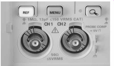
FIG.27 Most oscilloscopes state their input loading next to the BNC input
socket
The solution to the capacitance problem is to make a paralleled pair of potential dividers, one resistive, one capacitive (see FIG.28).
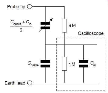
FIG.28 An oscilloscope probe is essentially two potential dividers in
parallel. The complete circuit is contributed partly by the oscilloscope, partly
by the ''probe''
The 1 M-ohm resistor is the standard oscilloscope input resistance, and this is in parallel with the oscilloscope's input capacitance and the lead capacitance. Together with the 1 M-ohm resistor, the additional 9 M-ohm series resistor forms a 10:1 potential divider. The cunning bit is the addition of the capacitor across the 9 M-ohm resistor. There are two ways of looking at this capacitor:
-- Potential dividers: The 9 M-ohm/1 M-ohm resistive potential divider has a loss of 10:1. We can also make potential dividers from capacitors, but because a capacitor's reactance is inversely proportional to its capacitance, a 10:1 capacitive divider requires the upper capacitor to be one-ninth the value of the lower capacitance.
-- Time constants: We can view the upper resistor/capacitor combination as a high-pass time constant, and the lower resistor/capacitance combination as a low-pass time constant. If the time constants are equal, their filtering effects cancel out and the network has a flat frequency response.
Looking into the input of the circuit, at DC the capacitors are an open circuit, so we see the two resistors in series, giving an input resistance of 10 M-ohm. At high frequencies, the capacitors are short circuits, so we can neglect the effect of the resistors, and we see a pair of capacitors in series:
At the expense of oscilloscope sensitivity, and by adding a resistor and capacitor at the far end of our lead, we have reduced the input capacitance by a factor of ten from 120 to 12 pF. Oscilloscope probes always state their input capacitance, either in the data sheet that came with the probe, or on their connector (see FIG.29).
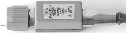
FIG.29 Some probes state their essential data on the connector housing
Because different oscilloscopes have different input capacitances, we need to be able to adjust the upper capacitor to suit the oscilloscope. This adjustment is often a small screw in the side of the probe (see FIG.30).
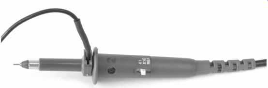
FIG.30 Probes are often equalized by a small screw in the body.
The adjustment is set by connecting the probe to the 1 kHz square wave provided by all oscilloscopes on their front panel, and often called Cal. The oscilloscope is set to display one cycle of the square wave, and the capacitor adjusted to give the flattest, squarest, leading edge (see FIG.31).
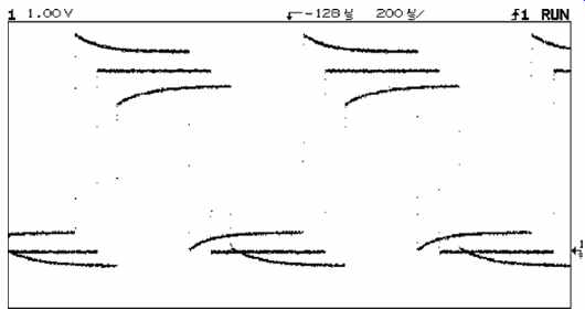
FIG.31 Correct probe equalization produces a square leading edge (middle
trace), rather than overshoot or rounding.