The use of crossover networks is based on the idea that two loudspeaker drivers
must be better than one. Although a great number of listeners achieve "acceptable" sound
using only one loudspeaker driver, the advantages of sharing the spectrum between
two or more specialized drivers seem obvious. The response should be flatter,
since each loudspeaker is required to perform well over a comparatively limited
range, and the cross modulation distortion should be lower, whether it is caused
by Doppler effect or simple amplitude limitation. Yet, the more one goes into
the problems of multiple speakers and the networks crossing over the signals
between them, the more remarkable it seems that they so often produce worthwhile
results, using the rough design methods most generally applied.
We propose below to approach the general problem of crossover networks from first principles, questioning the comfortable assumptions that are usually, and often unjustifiably made, hoping to reach a better understanding of the problems and through it, a more reliable method of design.
We will discuss the problem in its simplest form, crossing over between two loudspeakers, as in Fig. 1 (a). Three-way, four-, or five -way systems are best handled as trees which divide into only two limbs at any one time. Thus, the four-way system of Fig. 1 (b) divides, initially, into two paths for high frequencies and low frequencies. Then the high region is split once again into the mid highs and the upper highs, while the lows divide into the bottom lows and the mid lows. Thus, the problem is split into designing three separate two-way crossover networks.
Although we are discussing crossovers in general, I must here and now declare my preference in favor of passive crossover networks. The purpose of crossovers, either active or passive, is to shape the spectra of the signals to the two outputs or speaker drivers, and the same shaping responses will often be used with active and passive crossovers.
The active crossover has the advantage in that it can be changed with comparative ease. This is most useful when different driver systems must be handled, and particularly in experimental work. Besides, the same advantages of handling different parts of the spectrum in different devices apply to amplifiers, as well as to loudspeaker drivers, though with less force. Nevertheless, a high-quality amplifier is expensive, and with the cost nearly doubled for stereo and doubled again for quadraphonic, this makes one hesitant about doubling it yet again for bi-amping, even though I know that some will not agree with this. Perhaps, one day I will be satisfied that a bi amp pair using a common power supply can be made at a price similar to a single amplifier with equal ease. Then I may retract, but in the meantime... .
Even when a passive crossover uses large capacitors and inductors with large quantities of copper, it will always be lighter and less expensive than a second high -quality amplifier, and unless one is careless with the inductor core material, its linearity is beyond question. Besides, it is easily mounted out of sight in the loudspeaker cabinet.
With that opinion declared, we will now concentrate on the Butterworth -type responses invariably used in almost all passive crossover networks. Even so, Butterworth responses are the most widely used in active crossovers also, though by no means the only ones possible.
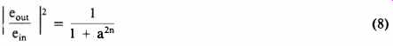
The response of a filter or any device in fact whose response varies with frequency, such as an amplifier, can be described by the ratio of its output voltage to its input voltage, in terms of a polynomial in w, the angular frequency, i.e. 2 π f,
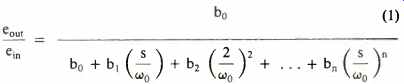
Any reader who feels threatened at this stage by such a long algebraic expression is begged for a little patience. If such algebra seems quite impenetrable, remember that there are many to whom Indian music, Haydn, Britten, or Prokofiev are equally unapproachable, and many more to whom they are a joy.
The above equation is at its most formidable because we have made it as general as possible. In fact, the b coefficients are simply numbers and they determine the shape of the frequency response. We vary the shape of the frequency response by varying the b coefficients.
Again, bo is often unity; if it is not we can divide through numerator and denominator to make it so. We then have a new set of b coefficients (b,/bo), (b,/bo), etc. The parameter wo is the angular form of the characteristic frequency fo such that

and it sets the position of the response in the frequency spectrum. For many purposes we would prefer the last term of the denominator in the form (s/w0,)", particularly when bo is unity, so we could rewrite the expression again in terms of a new characteristic frequency with
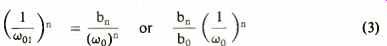
and readjust the other terms accordingly. This apparently trivial arithmetic manipulation can be a great help in getting the polynomial into a recognizable shape, and recognition of response shapes from the pattern of coefficients comes fairly readily once one is familiar with some of the basic polynomials.
Such manipulation is quite straightforward. Not long ago it was also very tedious, time consuming, and subject to human error, but nowadays it has become magically simple with the advent of electronic calculators, particularly the programmable ones. With s in the denominator, the expression is in the operational form that can be manipulated using the Laplace transform to give the transient response, the shape of the output waveform to any given input waveform. This is especially useful to engineers working in television or radar.
But in audio, where we are mainly interested in amplitude and phase response, we write jw for each s and equation 1 takes the form:
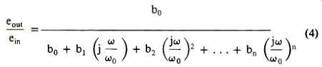
First because the expression (w/w0) appears so often and is a ratio, a pure number that is called normalized frequency, we allot it a symbol of its own

This makes things easier for the reader once he is used to it.
It is also a boon for long suffering typists and typesetters!
[Editor's Note: And editiors and proofreaders!] Now, j is the mathematical abstraction V--1. It was used by Steinmetz in a.c. theory to define quadrature or "imaginary" components, though their contribution is just as palpable as the in -phase, so-called "real" components. Then substituting in equation 5 and using the properties of j that j2 is -1, j3 is j, j4 is +1, and j5 is +j, and so on, and finally grouping "real" and "unreal" components, we can easily derive an expression for the phase angle ß between input and output:

and also the amplitude response in terms of the modulus squared:
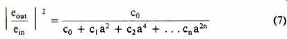
where co is obviously b20; c1, is seen to be b21-2b0b2, c4, is b2 2 -2b1b3 + 2b0 b4, and so on, with cn equal to b2 n.
Taking stock, we now have an expression for the amplitude vs. frequency response. This contains only even powers of a which we nominated in equation 5 as the frequency f "normalized" to a characteristic frequency fo, i.e. a pure number. The expression also contains the coefficients c0 c2 ... cn which again are pure numbers.
The highest power of s, and thus of a2, is n which is the "order" of the filter and also is the minimum number of reactances needed to make a filter in practice. Thus, one cannot build a third -order filter with fewer than three reactors, either two inductors and one capacitor or two capacitors and one inductor, or in the case of an active filter, three capacitors, along with suitable resistors.
The reader may have noticed that the response in equation 1 is unity at a low frequency when a is very small. It could denote either a passive or an active filter. Again, the response becomes smaller and smaller as a increases, obviously a lowpass filter.
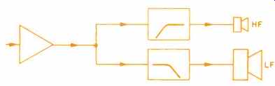
Fig. 1a-Dividing networks for a two-way system.
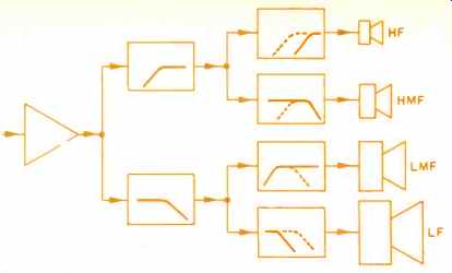
Fig. 1b-Dividing networks for a four-way system.
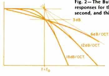
Fig. 2-The Butterworth responses for the first, second, and third order.
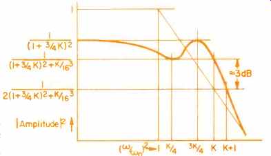
Fig. 3-Chebychev responses of the third order.
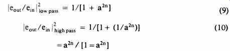
For a high-pass filter, (s/w0) in equation 1 is replaced by (wo/s). Then in equation 2, (jw/wo) would become (coo/h.)), and when equations 4 and 5 are applied to a high-pass filter, a becomes (1/a) in every term.
We have by now established the form of the amplitude response consisting of a single number numerator with a denominator that is an algebraic expression, a polynomial in powers of a2. A response can, of course, have polynomials in both the numerator and the denominator, and these are sometimes used in active crossovers, but we again limit our field of inquiry by ignoring such responses, for the moment at least.
In 1930, Butterworth (1) realized that if all coefficients in equation 7 are properly chosen, then the resulting amplitude response, now associated with his name,
has some rather special properties. First and most important, it is "maximally flat." In other words, the response in the pass band stays flatter longer than any other smooth, monotonic response of order n before it finally starts to attenuate. The squared modulus of the response passes through 1/2, i.e. is 3dB down, at fe and falls after that at a rate which tends more rapidly than any other to the ultimate, asymptotic, slope of 6n dB per octave, or if you prefer, 20n dB per decade.
While the Butterworth (maximally flat amplitude) response is the sharpest monotonic response of order n, it does not afford the fastest cut off around the transition frequency or the steepest slope in the region just beyond. Filters based on polynomials first described by Chebychev, or Tschebyscheff, or other spellings depending on how you prefer to transliterate Russian cyrillic script, produce a response which ripples at first, extends further out, and then attenuates more rapidly before finally taking up the same ultimate slope. The denominators include expressions which go to zero at some frequencies making the response ripple back to its d.c. value.
The manner in which the use of a Chebychev filter produces ripple, plus a widening of bandwidth plus a more rapid initial slope, is shown schematically in Fig. 2. But again Cheybchev filters are not used in crossover networks and we leave them too by the wayside. Interested readers are referred to ref. 2. The important point is that Butterworth shaped filters do not cut off as sharply as some other filter shapes of the same order, Chebychev filters, or even better Cauer filters, using elliptical functions. But they have the fastest cut-off of any monotonic, i.e. smooth, curve of that order.
However, the Butterworth filter has another advantage.
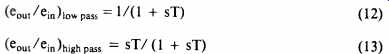
Suppose we divide the spectrum into two parts using a pair of Butterworth filters, one high pass and one low pass, but both with the same cut-off frequency, f0. Then we can write the two responses, again using a as the normalized frequency, the ratio between f and fa, as
Then summing the output powers from the two filters

Thus, a properly designed pair of Butterworth filters can divide the power from the amplifier into two bands without loss and also present to the amplifier a constant load impedance across the whole band. This can be seen graphically in Fig. 4. The familiar view (a) has both scales, for amplitude and frequency, plotted logarithmically. This shows well how each filter goes rapidly from the pass -band with flat response, to the stop band where the attenuation soon reaches a constant rate of increase of 6n dB per octave.
But with the same curves plotted in (b) on linear scales of power (i.e. of amplitude squared into a constant resistance), it is easier to see how the two power spectra are complementary and add to a constant sum at all frequencies.
This use of the whole power from the amplifier and the constancy of load impedance presented to the amplifier output makes the Butterworth filter ideal for crossover networks in general, especially passive ones. Again, the Butterworth shape is not the only one possible for a crossover network absorbing constant power. The Cauer or elliptical function filter allows a much more rapid transition from the pass band to the stop band, with a null response (given ideal components) not far into the stop band. However, it needs more reactive components. Thus, realistically, one must compare a Cauer filter with a Butterworth filter containing an equal number of reactances, capacitors and inductors.
Then, in general terms, with filters of the orders likely to be used, or afforded in loudspeaker systems, both Cauer and Butterworth filters give similar attenuations in the region of the following maximum, e.g. f4 for the low-pass filter in Fig. 1 (c) and f, for the high-pass filter. The attenuations of the Cauer filters are greater nearer the crossover, hence they are more tolerant of drivers with dubious response a little out of band. But, beyond f. (or f2) their attenuation is not so great, hence they are less effective, for example, in keeping down the excursions of the tweeter with lower frequency signals.
Besides their phase disturbance is greater. Thus, while one hesitates to rule out Cauer networks altogether, they seem to confer little advantage and have not been used, to my knowledge, in the past.
Butterworth -type crossover networks are shown in Fig. 5 in a form suitable for design. Cauer-type networks are shown in Fig. 6 for a comparison. Networks of orders up to three, as in Fig. 5, are likely to be most useful. However, fifth -order networks have been described (3) and are used by at least one manufacturer.
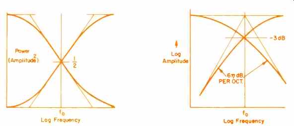
Fig. 4a--Responses of a Butterworth pair of filters with conventional scales--logarithmic
in amplitude and frequency.
Fig. 4b--Responses of a Butterworth pair of filters with a linear scale (i.e. amplitude squared) and logarithmic for frequency.

Fig. 4c--Responses of a pair of Cauer filters for comparison with linear scales
for power and logarithmic for frequency.
Amplitude Response of Summed Signal
We have seen that the sum of the powers out of a pair of Butterworth filters with the same cut-off frequency is constant. But it does not follow from this that the sum of their amplitudes, which depends on phase relationships as well, is constant also. When two signals of equal amplitude are added together, the amplitude of their sum will be twice, e.g. 6 dB higher, if they are in phase, only 3 dB higher if they are 90° apart, and will be zero, a null, if they are 180° apart.
So let us see what happens when we add the outputs of two Butterworth filters, high pass plus low pass. Consider first the very simplest filter order pair in which
...then the sum is:
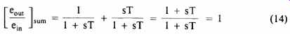
In other words, the response of the summed signal is completely flat across the whole band. Unfortunately, this is the only case in which the response is completely flat. Now consider what happens when we subtract two first order responses, i.e. we add them out of phase by reversing the connections to one driver. Then
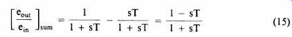
This is an all -pass response, i.e. its amplitude response:
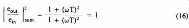
... is still quite flat, but now the phase angle between its output and its input

swings from zero at low frequencies to 180° at high frequencies. This can be considered alternatively as a time delay

which varies from 2T (T being equal to 1/(2 pi f0), e.g. 160 µS when f0 is 1 kHz) at low frequencies to zero at high frequencies. This involves us of course in the whole vexed question of time delay. Is it important? It has been pointed out before that a delay differential obviously does matter if it is large enough, if the highs arrive today and the lows arrive tomorrow. What then is the smallest delay difference than can be perceived? Is 320 µS, the time sound takes to travel 10 cm in air, important? Or half that? Or twice that? Again, if the delay is constant across the whole audio band and only reduces outside it, e.g. above 20 kHz, it obviously will not be heard.
But what when the center of the phase change moves down towards 10 kHz, or 5 kHz, or 2 kHz?
Tests undertaken by authorities as diverse as the Bell Telephone Laboratories many years ago, and more recently the German Post Office and Prof. Ashley seem to indicate that a delay variation of several milliseconds across the band cannot be heard in a monophonic signal. In stereo, on the other hand, delay differences of less than a millisecond between the two channels are quite significant because they move the position of the sound image.
But while delay differences of several milliseconds are most likely unimportant in an audio signal fed to a speaker system, they are important if they occur between two drivers in a two-way system over the frequency range of the crossover.
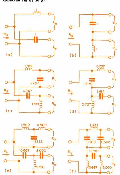
Fig. 5--Butterworth-type dividing networks. First order (a) parallel, (b)
series; second order (c) parallel, (d) series, and third order (e) parallel,
and (f) series. Component values are normalized for Ro = 1 ohm and wo = 1 radian/second.
For actual component values, multiply inductances by Ro / wo for Henries and
capacitances by 1/w0 Ro for Farads. Thus, when fo is 1 kHz (hence 1/wo is 160
microseconds) and Ro is 8 ohms, multiply inductances by 1280 µH and capacitances
by 20 µF.
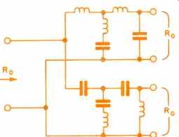
Fig. 6--A Cauer-type dividing network.
In this region, the two sound sources act together as a column which is comparatively directional, and any delay difference between them can easily swing the axis of the column response away from the listener. So, referring back to equations 14 and 15, we can say that while a pair of first-order crossover networks will produce a flat response across the band, it is only when the two drivers are connected in-phase that their combined response will be truly flat. When the drivers are connected out of phase, the amplitude response will be flat, but the overall signal will suffer more delay at the low frequency end of the band, 320 µS for a 1-kHz crossover and in inverse proportion for other crossover frequencies. The delay drops to half at the crossover frequency itself and zero at very high frequencies. Such a difference between the two connections is almost certainly inaudible. But one must remember that this is true only on the assumption that the two transducers are ideal. This is particularly hard to achieve with a first -order crossover because:
a) The amplitude and phase response of both drivers must be flat over a wide frequency range either side of the crossover frequency or the overall response will be affected.
Thus, if the responses of the two drivers had a 90° phase difference at the crossover frequency before the crossover network was connected, the overall result using the crossover network would be a 6 dB peak or a very deep notch depending on whether the phase shift was ± 90°. Even four octaves, i.e. 16 times, away from the crossover frequency, e.g. with a 1 kHz crossover frequency, at 62.5 Hz or 16 kHz a phase difference of 90° between the two driver responses would produce an amplitude disturbance of ±0.5 dB in the sum signal.
b) The woofer and tweeter should be physically close together, and the line joining their voice coils should be at right angles to the line between them and the listener, otherwise the column that they form at frequencies around the crossover may not "illuminate" the listener.
Of course, a steeper crossover slope reduces the out-of-band performance of the drivers. If we apply the summed signal test to a second-order filter (or any other even-order filter), we will find that there is no way to connect the drivers for flat response. However, third-order filters can provide flat response with some delay error, but in this case we find (again, assuming ideal drivers) that we should reverse the polarity of one of the drivers. (3)
Thus, we see that loudspeaker crossover networks should usually consist of complementary pairs of high-pass and lowpass Butterworth filters of the odd-order. The first-order response is the only one in which an ideal total response is achievable. The third-order response seems necessary when excursion of the upper driver limits power handling because of distortion or damage.
References
(1) S. Butterworth, "On The Theory of Filter Amplifiers," Wireless Engr., (October, 1930).
(2) A.N. Thiele, "Filters With Variable Cut -Off Frequencies," Proc. TREE Australia, (September, 1965; pp. 284-301).
(3) A.N. Thiele, "Optimum Passive Loudspeaker Dividing Networks," Proc. TREE Australia, (July, 1975; pp. 220-224).
(Source: Audio magazine, Aug. 1978)
Also see: Confessions of a Loudspeaker Engineer (Aug. 1978)
= = = =