The concept of frequency modulation ( FM) is not new, but only comparatively recently has it been commercially successful. Before the achievement of FM the type of modulation employed was amplitude modulation ( AM). So far as the majority of people even in the radio field were concerned, the only method of conveying intelligence from the transmitter was to amplitude modulate the carrier. The prevalence of this belief was only natural, because AM was the only form of modulation used in the past, and very little was known about other types of modulation. Even ten years ago, if one had made a survey and asked the question of how intelligence could be conveyed from the transmitter, the majority of replies, from others than engineers engaged in radio work, would have indicated use of an audio signal which varied the amplitude of the carrier. In short, it was not generally known that other forms of modulation could be used. Therefore, a thorough understanding of what is meant by modulation as applied to radio cannot but be helpful.
Modulation The primary purpose of radio broadcasting is to transmit intelligence. This intelligence finally appears as an audible sound at the receiver. In order that these audio signals may be received, they must be propagated through space by some special means. Audio signals by themselves cannot be radiated into space as electromagnetic energy and travel great distances. Some method must be used of helping to propagate the intelligence through space.
It wad known that signals far above the audio range could be propagated through space very easily in the form of electromagnetic waves.
These signals were referred to as radio-frequency waves (r.f.) or carrier waves and could be of almost any frequency, as long as they were of an r-f nature, and still be radiated. It was possible to use these r-f waves as a means of transporting the audio signals to the receivers. Briefly this was accomplished by superimposing the intelligence on the r-f wave (that is, the carrier) so that this new r-f wave had one of its characteristic features varied in accordance with the method of superimposing the intelligence. This superimposition of one signal on another is termed modulation, and the new wave is termed a modulated wave. This principle is well known to many, but its analysis is very necessary for fully understanding the topic of FM, as well as other types of modulation.
When a carrier signal of constant amplitude and power is generated by a transmitter without any intelligence superimposed upon it, it will be accepted by the receiver, but no information or audio will appear in the output of the set. The underlying principle behind transmission for the proper reception of intelligence is to use a carrier that can travel through space (that is, be propagated) and that can be varied somehow in accordance with the superimposition of the intelligence to be transmitted. This variation of the carrier can be accomplished by a number of methods which will soon be explained. In dealing with r-f carrier and other frequencies they all will be rep resented as sinusoidal in nature to facilitate the discussion.
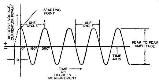
Fig. 1-1. Representation of a carrier wave which is varying sinusoidally,
on which its three characteristics, amplitude, frequency, and phase are
indicated.
In Fig. 1-1 an ordinary carrier signal which is varying sinusoidally is illustrated. The height of the signal is called its strength or amplitude. The strength of the signal between the maximum positive and negative peaks is referred to as its peak-to-peak amplitude. Consequently, amplitude is one of its characteristics. The time that part of the wave takes to complete one swing going through a positive and negative part of the signal and ending at the same level where it started is called one cycle of the signal. The number of times that the cycle repeats itself in each second is called the frequency of the signal, and it is expressed in some number of cycles per second. Thus, frequency is another characteristic of the signal. It may seem very elementary to indicate these well-known basic characteristics, but the purpose will be evident when the modulation of the carrier is analyzed under different conditions.
One more basic characteristic of a wave is its phase relation. This is a difficult concept to understand especially when only one signal is considered. If two different sinusoidal signals existing at the same point were compared, the idea of phase relations would be easily seen; however, this is not the situation in Fig. 1-1. In order to under stand the fact that, besides amplitude and frequency, phase is also an inherent characteristic of any alternating wave, some reference point has to be used. It is known that every cycle of frequency revolves through 360° with reference to the time axis. That is, by the time one cycle is completed it will have traversed 360°. The reference to 360° in every cycle is a concept that is very well known, and there is no necessity to elaborate any further about it. When the phase of a signal is referred to, it is usually related to some other signal, but when only one signal is under discussion, the start of the alternating motion of the signal is referred to an arbitrary set of axis.
In this respect the phase relation of a signal by itself can be understood.
When any graph is made, horizontal and vertical lines (set of axes) are assigned to represent the respective variables to be plotted. The same is true for a sine wave. A set of axes is used to indicate the true alternating motion of the wave with respect to all of the signal's characteristics. This is so in the wave of Fig. 1-1. The sine wave is seen to be alternating above and below a reference axis called the time axis or baseline. Its amplitude and frequency are readily noticed.
The wave shown is seen to be starting out, not at the crossing between the axis, but at the maximum amplitude of the signal. Since every half cycle represents 180° and every quarter of a cycle 90°, the signal shown in Fig. 1-1 is said to have a 90° phase lead. Consequently, it is seen that phase is one of the basic characteristics of any wave. Naturally, the phase relation can be zero degree.
In practice, when phase relationship is given, it is almost always made with reference to some other signal. This will be evident as this Section progresses. It will be seen later that there is a very close relationship between the frequency and phase of a signal.
The illustration of how simple it is to represent a signal in vector form at its starting point with relative phase is shown in Fig. 1-2.
The length of the vector A represents the magnitude or peak amplitude of the sine curve, whether it be voltage, current, or power. The displacement or direction of the vector from the 0° reference point is the relative phase of the signal, and it is seen to be 90° leading. If a quick representation of the instantaneous amplitude and phase relation of a signal is desired, the use of vectors will greatly clarify the picture. The use of vector representation is more thoroughly explained in the Appendix.
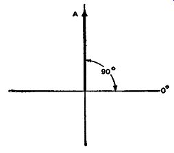
Fig. 1-2. The relative phase of the sine wave in Fig. 1-1 is shown vectorially
here by the vector A, being at 90° to the 0° axis.
It has been stated that to transmit intelligence a signal of radio frequency has to be used as the carrier for the intelligence. In order that this carrier properly support the intelligence signal, it has to be modulated by the intelligence signal. With respect to the radio field, modulation is attained by varying one or more of the three characteristics of the carrier (that is, its amplitude, its frequency, or its phase) in accordance with the instantaneous variations of some external signal which is superimposed upon the carrier. To realize the latter part of this statement fully, it must be remembered that the modulating or intelligence signal is also varying in accordance with time.
If the amplitude of the carrier signal is varied. in accordance with some superimposed audio signal, amplitude modulation or AM is attained. If the frequency of the carrier is varied, frequency modulation or FM is attained. If the phase of the carrier is varied, then phase modulation or p.m. is attained. Thus, any of three different types of modulation can be directly obtained. As distinguished from AM, the other two types of modulation are sometimes referred to as subdivisions of a modulation termed angular modulation. This terminology arises from the fact that angular relations undergo changes in both FM and p.m.
Amplitude Modulation
As pointed out in the preceding section, the three main characteristics of an r-f wave (as well as any signal) are its amplitude or strength, its frequency, and its phase. If an audio signal, for example, speech or a pure sine wave, is superimposed upon the r-f wave so that the amplitude of the r-f wave varies in accordance with the varying amplitude of the audio signal, then the r-f wave is said to be amplitude modulated. In other words, the combination of the modulating signal, which is the speech, the music, or the information to be conveyed, with the radio signal, is accomplished in such a manner that the modulating signal alternately increases and decreases the amplitude of the radio signal; this variation takes place at a rate determined by the frequency of the audio signal. The extent of this change in carrier level depends upon the relative magnitudes of the audio and the carrier signals at the instant they are combined.
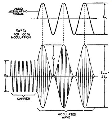
Fig. 1-3. The peak amplitude of the audio modulating signal is equal
to the peak amplitude of the carrier wave, resulting in the carrier being
100 percent amplitude modulated.
Neglecting the degree of modulation at the moment, let it be said that the stronger the audio signal combined with the carrier, the greater is the change in the amplitude of the carrier. This is of particular importance because the degree of modulation depends upon the amount that the carrier amplitude is changed. If the strength of the audio signal is such that its peak-to-peak amplitude is equal to the peak-to-peak amplitude of the carrier, 100 percent modulation exists.
(The peak amplitude of one is equal to the peak amplitude of the other.) This 100 percent a-m wave is illustrated in Fig. 1-3. If the peak amplitude of the audio signal is less than the peak amplitude of the carrier, the modulation that exists is less than 100 percent.
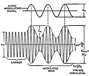
Fig. 1-4. The peak amplitude of the audio modulating signal is one-half
the peak amplitude of the carrier, resulting in a 50 percent a-m wave.
Compare with Fig, 1-3.
In Fig. 1-4 is shown an a-m wave that is 50 percent modulated.
That is, the peak amplitude of the audio is equal to half the peak amplitude of the carrier. As stated previously the instantaneous amplitude of the audio signal adds to or subtracts from the instantaneous amplitudes of the carrier resulting in an a-m signal.
Modulated signals for 100 percent modulation and below have been shown in Figs. 1-3 and 1-4. However, a different type of waveform exists when the amplitude of the modulating signal is greater than that of the carrier. This is termed overmodulation, and a picture of an over-modulated wave is illustrated in Fig. 1-5, together with the modulating signal. It will be noticed that an overmodulated wave is not continuous and as such does not result in the full reproduction, upon demodulation, of all the audio signal. This results in distortion in the output of the receiver.
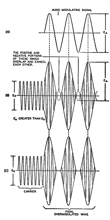
Fig.1-5. When the peak amplitude of the modulating wave (A) is greater
than the amplitude of the carrier wave, the resulting modulated wave
(C) is said to be overmodulated. Notice that the resultant overmodulated
wave is not continuous, which means that the output of the receiver will
be distorted.
To determine the percentage of modulation of a signal (not over modulated) viewed on an oscillograph and having the type of pattern shown in Figs. 1-3 and 1-4, the following simple procedure should be followed: Measure the maximum peak-to-peak amplitude of the modulated signal. This is designated as Ema,; as shown in Fig. 1-4. Next measure the minimum peak-to-peak amplitude of the modulated signal. This is designated as Em,n as seen in Fig. 1-4. Then to determine the percentage modulation the following expression is used:

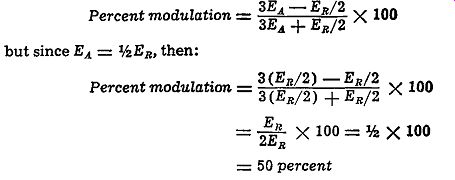
For instance, in Fig. 1-4 the Emaa, is equal to 3E.4. and Emt,. is equal to E 11,/2. Therefore, d l
When percentage modulation is computed from directly viewing a picture on the scope, the measurements are used directly. For instance, if a picture of a modulated wave was such that Emaa, measured 1.5 inches and E_min measured 0.5 inch then:
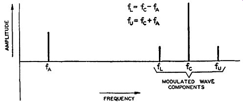
Fig. 1-6. In this spectral distribution of a 50 percent a-m wave, f
A is the modulating signal, which is one-half the amplitude of the carrier
component, f c.
The upper and lower sidebands, f u and f u are the sum and difference of the modulating and carrier frequencies, their amplitudes being ½ off. 1-
Certain very significant details are associated with such a-m waves.
First, the modulated wave is not of constant amplitude; in fact it is anything but constant, varying definitely with the amplitude of the audio signal. The second detail is that the composition of such an a-m wave consists of the carrier frequency and a series of other frequencies representing various plus and minus combinations of the carrier and the modulating frequencies. The modulating signal is considered as consisting of a number of frequencies because, when modulating a carrier with speech, the audio signal is definitely not composed of a single frequency but of a host of frequencies through out the audio spectrum. These combinations represent the sidebands of the carrier. The higher the frequency of the audio signal used to modulate the carrier, the greater is the extent of the sidebands. A spectrum picture of the component waves of an a-m signal is shown in Fig. 1-6. The carrier frequency is designated as fa and the frequency of the sinusoidal audio as fA• The upper and lower sideband components of the modulated wave are designated as fu and fL respectively. If the frequency of the carrier is 1000 khz and the frequency of the audio 5 khz, the upper sideband will be 1000 + 5 or 1005 khz and the lower sideband will be 1000 - 5 or 995 khz. The modulated wave is then said to cover a band of frequencies equal to the difference in frequency between the sideband components, and in the foregoing case the bandwidth is equal to 10 khz. It is, therefore, seen that the sideband components of the modulated wave are the portions of the signal that contain the intelligence.
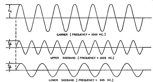
Fig. 1-7. When a carrier is 100-percent amplitude modulated, the amplitudes
of the upper and lower sidebands are each one-half the amplitude of the
carrier.
For 100-percent modulation, the upper and lower sideband component frequencies of a sinusoidally modulated wave have their amplitude equal to half the amplitude of the carrier. For 50-percent modulation both sideband components of the modulated wave have their amplitude equal to one-quarter of the carrier amplitude. The component waves for a 100-percent and 50-percent sinusoidally modulated carrier are shown in Figs. 1-7 and 1-8 respectively. In AM only two sideband components exist for each sinusoidal component of the modulating intelligence. This can be proved mathematically, but it is sufficient to say at this point that this condition does exist.
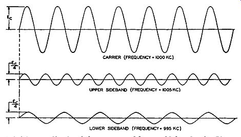
Fig. 1-8. The amplitude of the upper and lower sidebands of a 50-percent
amplitude modulated carrier are one-quarter that of the carrier.
A very important situation prevails in the components of an a-m wave in regard to power. For 100 percent modulation the power in the sidebands is equal to half the power of the carrier. Since the carrier does not contain any intelligence, the power in the carrier is wasted and only that in the sidebands becomes usable upon demodulation. Consequently, of the total power involved in 100 percent AM, only one-half is considered as utilized in reproducing the audio intelligence. That is why in AM 100 percent modulation is generally considered the best for maximum power transfer. In a 50 percent a-m wave, the power in the sidebands is only one-eighth of that contained in the carrier.
Though the a-m .form of transmission has been used for a long time, certain disadvantages have been continually apparent. One of these is the natural and man-made static problem. This was caused by the effect of such disturbances upon the received signal. Investigation disclosed that, when such electrical disturbances combined with the electrical wave in the receiver, the result was a change in amplitude of the carrier, just as if this disturbance were an audio modulating voltage. With the conventional receiver designed so that it responded primarily to variations in amplitude of the carrier, the elimination of noise became an extremely difficult problem.
In fact, under certain conditions when the noise-to-signal ratio was high, any attempt to remove or even decrease the noise, removed or decreased the signal as well. At times the noise reached such proportions that actual operation of the communication or broadcasting system was impossible. The search to alleviate the situation embraced many operations, such as selecting higher carrier frequencies, the development of noise-reducing circuits, municipal ordinances for filtering of noise-producing apparatus, the use of higher power at the transmitters, and even changing the type of modulation. This latter change was the most radical of the group because it involved a completely new type of transmission, and it really received its due consideration only recently, Frequency and Phase Modulation At the beginning of this Section it was shown that, besides the amplitude, the frequency and phase of the r-f carrier also could be varied in accordance with a modulating signal. Hence, FM and p.m., as well as AM, are possible. When the frequency of the carrier is varied directly, then the type of modulation is known as direct FM When the phase of the carrier is modulated, the type of modulation is known as p.m. or sometimes as indirect FM In the process of directly varying the frequency of the carrier, the phase is indirectly changed, and likewise, while directly varying the phase, the frequency indirectly changes. These facts will become evident in later sections of this guide.
Since direct FM and p.m. changes are related to each other, it is readily seen why they both are often referred to as FM in the broad sense of the term.
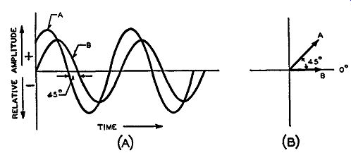
Fig. 1-9. Wave A has a greater amplitude than Band leads B by 45°, as
indicated. The vectorial representation of these two waves is shown in
(B) where the larger vector A is shown leading B by 45 °.
[To be more specific there are in reality three types of modulation with respect to frequency modulation. There are direct FM, indirect FM (a form of p.m. such as that used by Armstrong), and direct p.m. However, direct p.m. is utilized very rarely and consequently will not be considered in detail. Many of its effects and attributes are like those for indirect FM]
The purpose of either of these types of modulation is the same. That is, they both produce similar effects in that the FM receiver does not respond to changes in amplitude, and thus elimination of most types of noise interference associated with AM results. It should be remembered, however, that the modulating signal in either case directly produces changes in frequency or phase and not in amplitude.
Phase Modulation
This type of modulation is more difficult to comprehend, because in order to understand it the concept of phase has to be fully grasped.
It already has been stated that the concept of phase and phase difference is generally used with reference to two or more quantities. In Fig. 1-9(A) are shown two sine curves of different amplitude, with curve A larger in amplitude than curve B and leading curve B by 45°. In other words, the two curves are 45° out of phase with each other. The relationship between these two curves is illustrated vectorially in Fig. 1-9(B). The lengths of the vectors represent the individual peak amplitudes of the curves, and the angular separation between them shows their phase relation. With such vector representation the phase relationship and the relative strength of their signals can be readily noticed.
In p.m. the phase of the signal is varying, but at any one instant of time there exists a phase difference between these two signals which can be represented vectorially. In Fig. 1-1, it was shown that the carrier alone has a certain fixed phase relation designated as (θ, (the Greek letter theta). This fixed phase relation is often called the relative phase of the system. It is around this relative phase that the phase changing occurs to bring about p.m. directly; and this change is varied in accordance with the modulating signal. The methods of producing p.m. will be discussed later, but at the moment the realization that p.m. can exist is the important factor. Since it is a change in phase about the relative phase of the carrier that produces p.m., the relative phase under p.m. does not remain fixed. As the phase is no longer fixed, at any one instant of time an instantaneous phase has to be dealt with. The instantaneous change in the phase of the modulating signal changes the relative phase of the carrier in accordance with the modulating signal. Consequently, the variations in phase of the carrier convey the intelligence superimposed by the modulating signal. The phase is not constantly advanced in only one direction.
What happens is that the phase undergoes a cyclic change. That is, it undergoes an oscillatory motion in that it advances up to a certain point and returns. The phase swing or phase excursion can undergo hundreds of degrees o£ change.
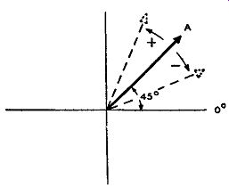
Fig. 1-10. A carrier that is phase modulated may be represented by a
vector A, which has a relative phase angle of 45° and is constant in
length. Phase deviation results when the vector varies above and below
its relative phase angle as indicated by the dotted vectors.
This phase swing or phase excursion is sometimes known as phase deviation and can be simply illustrated by the use of a vector dia gram. Let the relative phase of some carrier be equal to 45° with respect to some initial reference point as shown in Fig. 1-10 where the vector is represented as A. If the modulating signal is such that it alternately changes the instantaneous phase of the carrier, the phase of the carrier is in effect varying about its relative phase angle. When the modulating signal changes the phase of the carrier at any one instant in the negative or decreasing direction as indicated in Fig. 1-10, then, after it has reached its maximum swing in this direction, it will return to its former starting position and then swing in the positive or increasing phase direction. After it has reached its maximum positive swing it will return to its starting position to complete one cycle of phase deviation. Although the vector diagram visually takes into account a maximum of 360°, it should be understood that a phase swing a hundred or more times as many degrees is possible.
That is, the time lag between the relative phase of the carrier and that of the modulating signal is such that the vector A of Fig. 1-10 could swing in the negative or positive direction (as the case might be), so that the swing would encircle the 360-degree coordinate plane a number of times. After it had reached this maximum negative swing, it would return to its original starting position, still traversing the same number of revolutions about the axis. After reaching the starting position, it would swing in the positive direction the same number of revolutions as it did in the negative direction and then return to its starting point. In this manner hundreds of degrees of phase shift are encountered during only one alternation or cyclic change of phase shift. The actual value of the original reference phase angle in reality has nothing to do with phase modulating the carrier.
As its name implies, it is nothing more than a reference point about which the carrier becomes phase modulated.
Vector A in Fig. 1-10 represents the unmodulated carrier. If the carrier were amplitude modulated, the length of the vector would change. If the carrier were frequency modulated, the original frequency would change in accordance with the modulating signal, and the vector would rotate with a varying angular velocity dependent upon the modulating signal. In p.m. the phase varies about the relative phase of the unmodulated carrier; this movement makes the vector swing back and forth. At any one instant of time during the phase excursion the equivalent instantaneous frequency does not re main the same. If the vector rotates back and forth through a certain number of degrees, then at each instant of time during the swing the equivalent instantaneous frequency is changing. This is so because a phase change is equivalent to a change in instantaneous frequency, because every cycle of frequency change undergoes a 360-degree revolution. It is consequently seen that p.m. indirectly causes a change in the equivalent instantaneous frequency, thus indirectly causing FM The reverse is also true and will soon be evident.
Equivalent Frequency Change
To visualize the effect of p.m. causing an equivalent change in frequency more easily, the following analysis between two sine waves will be considered: Imagine two sine waves A and B, each 1000 cycles and secured from two different sources. Further imagine that the currents of these two sine waves are applied to a common resistive circuit, but by some means, after having started the two waves in phase, the phase of B is changed by varying degrees until B lags A by a maximum of 15°. This is shown in Fig. 1-11.
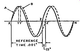
Fig. 1-11, left. Of the two 1- khz waves, A is the reference wave and
leads B, as the latter has passed through a variable delay network, which
lowers its frequency to 960 cycles at point Z'. At point N, the waves
are again at 1 khz as they were at the start.
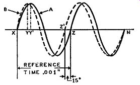
Fig. 1-12, right. The same 1- khz waves as in Fig. 1-11 are shown here,
but A, the reference wave, lags wave B, as the frequency of the latter
has been increased so that at point z, it is 1043 cycles.
Both frequency changes in these figures are effected by phase shifting.
An analysis of this drawing will reveal that the time required for the completion of a cycle of A is indicated upon the time axis as the reference time of 0.001 second. When we change the phase of one wave with respect to another and one wave lags the other, the second wave moves through whatever reference points are selected after the first; therefore, we can say that wave B at any instant is slower in time than wave A. This is evident in Fig. 1-11 as is the fact that the frequency of wave B slows down more and more as it approaches the completion of its cycle.
Such a phenomenon may appear confusing; but, if it is recognized that phase shifting circuits are available, that wave A is secured from one source and wave B from another source, and that B is passed through a variable delay network, the presence of two such waves of current of varying phase applied to a resistance network can be visualized.
Since frequency is expressed in terms of time, wave B, which is being subjected to a shift in phase with respect to wave A, is at any instant representative of a different frequency with respect to wave A. Thus, if we consider wave A as the standard reference of time with Y as the first instantaneous reference point, we note in Fig. 1-11 that this point is the peak of the positive alternation of A. However, wave B which started concurrently with A, has not reached its positive peak at Y, but does so at point Y'; therefore, in terms of frequency, B is slower than A. Later in the cycle, say at Z', for example, where wave B lags wave A by 15°, a greater amount than at Y and Y', wave B is still lower in frequency than before. The 15-degree difference is equal to 15/360 or 1/24th of the entire cycle. The time that it takes wave B to reach Z' is equal to one period (or one cycle of time) plus 1/24th of a period.
The period T, is referred to the starting frequency of 1000 cycles, and it is equal to 1/f where f is the starting frequency. However, at point Z' the frequency of B has changed (become slower), and the new period is equal to the old period plus the additional time required to traverse the extra !/24th of a cycle. Consequently, the total period for wave B at point Z' is as follows.
Total period= T + 2 1 4 T = ;!T
Since the period is equal to the reciprocal of the frequency, the equivalent instantaneous frequency of wave B at point Z' is 24 X f = 24 X 1000 cycles= 960 cycles 25 25
As the waves advance the phase difference between wave A and wave B becomes less and less, hence in accordance with what was said the equivalent instantaneous frequency of B is increasing, until, at point N, the waves are in phase and the equivalent frequency of B is the same as that of A, or 1000 cycles.
With wave A still the reference wave. suppose that the phase of B again is gradually changed with respect to A, but that B is now speeded up so that it leads wave A. This is shown in Fig. 1-12 where waves A al\d B, still beginning at 1000 cycles each, are in phase at X but at Y and Y' wave B leads A. If the curves are examined, it will be found that while wave A completes a cycle in 0.001 second, wave B has passed through more than one complete cycle in the same period; therefore, whatever the frequency of B, it must be higher than A. At point Z', wave B leads wave A by 15°. The equivalent instantaneous frequency of Bat point Z' is figured as in Fig. 1-11. The period that it takes wave B to reach Z' is I/24th of a cycle less than the reference period of 0.001 second. Therefore, the new period of B represented by point Z' is equal to the old period (reference period, call it T) less I/24th of this old period. Therefore, Period of wave B at Z' = T - ..!_ T = 23 T 24 24
Since frequency is equal to the reciprocal of the period, the equivalent instantaneous frequency of wave Bat point Z' is:
!! X f = ~! X 1000 = 1043 cycles
At N, both waves are in phase, and the frequency of B is the same as that of A. Referring again to Figs. 1-11 and 1-12, they illustrate how, by changing the phase of a wave, which is equivalent to slowing down or speeding up the wave, it is possible to create the equivalent of an instantaneous change in frequency. It should be stressed that the greatest significance of the examples given lies in the presence of a wave wherein the frequency is raised and lowered. A standard reference wave of fixed frequency is included only to illustrate properly how phase shift is equivalent to a change in the frequency.
Briefly summing up the basic characteristics of p.m., we find that the amplitude of the unmodulated carrier and the mean carrier frequency remain fixed, but the carrier undergoes phase variations (about its relative phase angle) caused by the modulating signal.
That is, in p.m. the equivalent instantaneous frequency undergoes cyclic changes about the mean carrier frequency due to the relative changes in the phase of the carrier signal. A more detailed analysis of p.m. will be discussed in Section 3 where the circuit for a basic p-m modulator is studied.
Frequency Modulation
In discussing p.m., it was brought out that indirectly the instantaneous frequency of the carrier was also changed: a change in phase produced an equivalent change in the instantaneous frequency, In frequency modulating the carrier, it is this instantaneous frequency which is varied directly, which in turn produces an equivalent instantaneous phase shift. That a change in the instantaneous frequency does cause this indirect change in the phase can be shown by analyzing Figs. 1-11 and 1-12 from the standpoint that it is the instantaneous frequency of wave B which is changed, with wave A remaining fixed as the reference wave. It would follow that a change in the frequency causes a change in the period, which results in a phase shift. Consequently, the converse statement that direct FM causes indirect p.m. is true.
It is very difficult to tell the difference between an FM wave and a p-m wave as they appear on an oscilloscope. This is best illustrated by showing pictures of both FM and p-m waves. Fig. 1-13 shows a p-m and an FM wave, both modulated by audio. In both types of modulation the modulating signal, wave A, is exactly the same in frequency and amplitude and so are the carriers of the respective modulated signals. The FM wave is shown at (B) and the p-m wave at (C). Two cycles of audio (represented by a sine wave) modulate both carriers as shown. The modulating audio signal is lined up with the modulated signal in order to show the effect the positive and negative half cycles of the audio signal have on the modulated waves.
In both modulated waves the modulation starts at the beginning of the audio signal, points R and R', and finishes at the end of the second cycle of the audio signal, points Z, Z', respectively. To the left of both of these signals, the rest of the signals at (B) and (C) represents the unmodulated carrier.
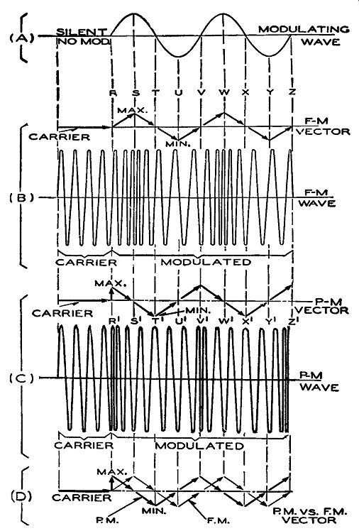
Fig. 1-13. The audio wave at A modulates the same carrier, shown to
the left of R and R', in such a way that the resultant wave at (B) is
frequency modulated and at (C) it is phase modulated. Above each of these
modulated waves is their vector representation, these being combined
at (D) for comparison. Note especially where the frequency is increased
and de creased in each modulated wave, as indicated by the respective
bunching or spreading of the individual cycles.
In the FM wave at (B) the frequency of the signal is being altered.
At the positive halves of the modulating signal the frequency of the FM wave is increased. This increase in frequency occurs between points R and T and between points V and X, with maximum frequency increase occurring at points S and W respectively. At the negative portions of the modulating signal, the modulated FM wave is seen to decrease in frequency. This decrease occurs between points T and V and between points X and Z, with maximum frequency de, crease occurring at points U and Y. The maximum frequency increase and decrease occur at the maximum amplitudes of the positive and negative half cycles of the audio modulating signal respectively. The frequency change as caused by directly frequency modulating a wave, as shown at (B) of Fig. 1-13, is, therefore, readily noticed. To illustrate more vividly the frequency changes of the FM sine wave, we have included above the wave a vector diagram showing how these frequency changes occur with respect to the audio modulating signal.
From this vector diagram the points of maximum and minimum frequency are readily noticed. Where the vector crosses the baseline, the frequency of the FM wave equals that of the carrier.
Now let us examine the p-m wave, part (C) of Fig. 1-13. If this p-m wave appeared on the scope, it would be difficult to tell whether the modulation was one of frequency or of phase. The changing of frequency of the wave which is caused by directly phase modulating the signal occurs as follows: At the beginning of the p.m., point R', the frequency of the wave suddenly changes. In fact, at point R' the frequency is a maximum as witnessed by the close bunching of the wave shape and as indicated by the p-m vector above the wave. As we proceed away from R' toward S', the frequency decreases and at point S' it reaches the frequency of the carrier. From point S' to point T' the frequency is continually decreasing, until at point T' it has decreased to its maximum value. This has occurred, so far, with respect to the positive half of the audio signal. Compare it with that part of the FM wave and the difference between both types of modulated waves manifests itself.
From point T' to point U' of the p-m wave, the frequency starts to increase again, until at U' the frequency has reached that equal to the carrier again. From point U' to point V' the frequency starts to increase (above that of the carrier), until at point V' it has reached its maximum value, equal to that at the previous point R'. From point V' to point Z' the wave repeats itself exactly as between points R' and V'. In other words, between points R' and V' one cycle of audio modulating signal has been traversed, and the same thing occurs for both audio cycles. Similar to the FM wave a p-m vector is drawn above the p-m wave better to illustrate the frequency changes that occur in the p-m wave. The composite picture of the p-m signal discloses that during the reversal of the audio modulating signal from the positive half cycle to the negative half cycle, the decrease in frequency is at its maximum. If this same point (T or X) of the FM wave is examined, it will be noted that the frequency here is equal to that of the carrier. From the p-m wave at (C) and the modulating signal at (A) it is seen that, when the audio modulating signal reverses from the negative half cycle to the positive half cycle, at points V' or Z', the increase in frequency is at its maximum. If these same points of the FM wave are examined, it will be seen that frequency is equal to that of the carrier.
One can readily understand how easy it might be to misinterpret a p-m wave as an FM wave, or an FM wave as a p-m wave. The drawings of the FM wave and p-m wave are shown only for comparison purposes, and they are exaggerated to procure a better picture. That is, the amount of increase or decrease of frequency in either case for the same audio signal and carrier is really not necessarily the same.
For an over-all comparison between the FM and p-m waves, a composite picture of both vector diagrams is drawn in part (D) of Fig. 1-13. This readily reveals that the relative changes in frequency for an FM and a p-m wave, for the same audio modulating signal and carrier, do not occur at the same instants of time.
Comparing FM with AM, the chief contrast is that in FM (as in p.m.) the amplitude of the modulated wave remains constant, whereas in AM it varies. In FM the carrier frequency is varied by means of the modulating signal. It is varied in such a manner that it undergoes frequency deviations on either side of its center frequency. These frequency deviations, or frequency swings, are dependent upon the level of the audio modulation, which means that the loudness or amplitude of the audio modulating signal is a determining figure in the frequency swing or deviation about the center frequency. The stronger the audio signal, the greater the change in frequency, but the amplitude of the FM wave is always constant. This is in contrast to the a-m wave, which is produced when the amplitude of the modulating signal varies the amplitude of the carrier. The frequency of the modulating signal in FM determines the number of times per second that the change or deviation in frequency of the carrier takes place. The higher the frequency of the audio or modulating voltage in the transmitter, the greater the number of times per second the carrier frequency changes between the limits determined by the amplitude or strength of the audio signal. This will be made clearer in Section 2 when the analysis of different FM wave shapes is considered.
In AM it was simply shown what was meant by percentage of modulation. It was also indicated that only two sidebands appear in AM, namely the upper and lower sideband, the frequencies of which are, respectively, the carrier plus the frequency of the modulating signal and the carrier less the frequency of the modulating signal. In FM, as well as in p.m., the percentage of modulation and the sideband characteristics are not so simple as in AM For instance, in FM if we were to refer to 100 percent modulation similar to the way percentage of modulation is understood in AM, the frequency swing of the FM wave would have to be such that it covered the whole of the carrier frequency on either side. We know this to be a practical impossibility, so the percentage of modulation in FM is defined in another way with respect to the deviation of the signal. This will be shown in the next Section.
Numerous sidebands may appear in FM as compared with only one pair in AM These sidebands are paired equally on either side of the center frequency. The sidebands nearest this center frequency and on either side of it are equal to the frequency of the carrier plus or minus the audio modulating frequency. The sidebands of the next nearest pair are equal to the carrier frequency plus or minus twice the frequency of the modulating signal, and so on with the other pairs of sidebands. In other words, the sidebands in FM are removed from each other by some integer multiple of the modulating frequency, and it is their strength which determines those that are effective in reproducing the modulated signal. As in AM, the intelligence of the FM signal is carried in its sidebands. The relative strength or the amount of the effective sidebands is determined by the degree of modulation.
Due to the number of sideband components in an FM wave, the required bandwidth for this type of modulation may be greatly increased as compared with AM This will all be evident from the more thorough discussion of FM waves in the next Section.
The FM and P-M Transmitter
Many different types of so-called FM transmitters are in use today.
The two main types are those using direct methods of FM and those using indirect FM, or p.m. The methods of obtaining the modulated signal differ in both of these systems. However, as far as the reception of signals is concerned, both types of transmitters are considered as equivalently transmitting FM This is easily understandable since it was shown how a p-m signal indirectly undergoes changes in its equivalent instantaneous frequency The performances within either type of transmitter, from the viewpoint of desired and undesired characteristics, is quite different. That is, the basic operation of producing the correct type of modulation differs appreciably enough to warrant discussion of the various transmitters. Since a-m transmitters are most familiar, wherever possible, comparisons between the a-m and FM systems will be included in order to correlate certain fundamental relations.
It is quite difficult to draw general block diagrams of a-m transmitters and of FM and p-m transmitters that will represent the only types in use, because there are so many versions of such transmitters, even though the FM and p-m types are virtually new in the field of radio broadcasting. The block diagrams shown in this section are chosen to be indicative of the general run-of-the-mill transmitters.
The components that are included are necessary for the basic operation of each type of transmitter and also for the comparison of the individual transmitters.
Fig. 1-14 shows three block diagrams of a-m, FM, and p-m transmitters. Part (A) of Fig. 1-14 is that representing an a-m transmitter. It is the familiar type wherein the r-f section consists of an oscillator feeding into a buffer, which in turn feeds into a system of intermediate power amplifiers and/or multipliers which in turn feed into the final power amplifier stage. The audio system consists of the mike and speech amplifier which feeds into the modulator system. For high level (plate or grid modulation) a-m transmission, the output of the modulator is usually fed into the final power amplifier stage, as indicated by the solid line leading into the last stage, whereas for low level a-m transmission the output of the modulator is fed into some-intermediate amplifier stage as shown by the dashed lines. The modulating power needed in either type of a-m transmission is far in excess of that required for modulation either in FM or p.m.
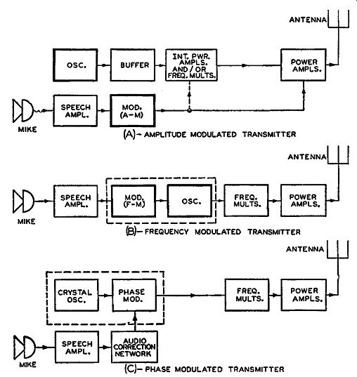
Fig. 1-14. Block diagrams of a-m, FM, and p-m transmitters are shown
in (A), (B), and (C) respectively.
Parts (B) and (C) of Fig. 1-14 show the block diagrams for the FM and p-m transmitters, respectively. If the block diagrams of the three different types of transmitters are examined it will be noticed that there is not much difference as far as their r-f sections are concerned.
All three require oscillators, intermediate stages usually consisting of frequency multipliers or amplifiers, and the final power amplifier stage. The greatest difference among them would appear to be in the method of modulating the carrier. It must be remembered, however, that we are looking at the block diagram views of the different transmitters and are not really considering their internal structures. The r-f sections up to the final power amplifier do differ appreciably as far as their construction is concerned. In most a-m transmitters ( especially of the high level type), the r-f tubes used are of the power variety, whereas in FM and p-m transmitters, they can be (and often are) of the receiving tube type. Consequently, in viewing block dia grams it should be understood that as far as similarities exist, they exist in the functioning of the different stages and not necessarily in the methods of performing these functions.
The primary difference between the operation of the FM and p-m transmitters lies in the methods of producing the modulation. In the FM transmitter, the output of the speech amplifier is usually fed directly into the modulator stage. The modulator stage injects a variable reactance into the oscillator stage changing its frequency in accordance with the varying reactance. The output signal from the oscillator is thus frequency modulated. It is sent through a system of frequency multipliers in order to obtain the correct deviation and frequency output.
In the p-m transmitters (indirect FM), the audio signal is fed into some type of so-called audio correction network before it is fed to the phase modulator. This audio correction network makes the p.m. that occurs directly proportional to FM The phase modulator works in conjunction with a crystal oscillator so that, when an audio signal is applied to the microphone and, hence, to the modulator, the phase of the crystal oscillator signal is varied in accordance with the audio modulating signal The output from this oscillator-modulator network is then fed into a series of multiplier stages. There are numerous types of indirect FM transmitters which utilize different methods of phase shift, and they are discussed in detail in Section 4.
The frequency multipliers used in a-m transmitters are primarily intended to increase the fundamental frequency put out by the oscillator. The oscillator itself does not produce the transmitted frequency, because it is more stable at lower frequencies than at higher frequencies. Since in FM and p-m transmitters the final transmitted frequencies are in the 88-108 mhz range, this fact becomes even more important when considering them. The frequency multipliers used in FM and p.m. are employed not only to increase the fundamental frequency put out by the oscillator but also to increase the frequency deviation (or phase shift). This will be clarified later in this guide.
In all three types of transmitters the final power output stages are chiefly used to increase the power of the modulated signal before transmitting it. In the high level type of AM, as mentioned previously, this last stage is modulated, but in FM and p.m. it is not. This last stage in all cases has to be properly matched to the antenna for the maximum transfer of energy.
The antennas of the FM and p-m system are important in that they have to be directional. As the propagation of energy from FM transmitters is at the higher frequencies (it is in the 100 -mhz region since the frequency allocations have been changed from the old band), then the special effects of the different layers of the atmosphere have to be taken into account. The erection of FM antennas is such that their height and the type of radiators used are very important problems.
That is, the antenna should be as high as possible. Likewise, the radiators have to be in certain positions in order to propagate the energy in the correct direction. This will be discussed in greater detail in Section 5.
Relative Factors in the Transmission of FM Signals
Until very recently the frequency band of FM 4 war between 42 and 50 mhz. This band covered only 8 mhz and, naturally, the allotment of the number of stations per given area was not many. The relatively increasing importance of this type of modulation led the Federal Communications Commission (FCC) to allot a new band in the frequency spectrum to FM. This new band, in effect since 1946, is between 88 and 108 mhz. (The top two megacycles of this band are re served for facsimile.) These new frequencies, as well as the old band, are in the so-called v-h-f region (very high frequency), and transmission at these frequencies presents a different problem from trans mission at the frequencies of the a-m broadcast band.
Long before FM came into use, high-fidelity broadcasting was almost always desired. From 550 khz to 1600 khz a-m broadcast stations are separated by 10 khz. No two stations on adjacent channels occupy the same service area, unless their transmitted power is quite weak. Modulation frequencies as high as 7.5 khz can now be used. An a-m station can use frequencies higher than 7.5 khz provided its transmitted signal does not interfere with any other station. However, not many stations operate even as high as 7.5 khz and few operate higher, any system that can always transmit a signal modulated to 15 khz with minimum distortion will be the best high-fidelity system.
---------
When FM antennas are mentioned they shall be understood to include those used for both the direct FM and indirect FM (p-m) form of transmission.
In most cases when the term FM is used without specifying whether direct or indirect FM (or p.m.) is meant, it encompasses both types.
------------
Frequency modulation properly used achieves such a system. By transmitting in the v-h-f region, the separation, or bandwidth, between stations can be greater than that usually found in the a-m broadcast band. In fact, the bandwidth, or separation, between channels in FM is a minimum of 200 khz. It must be realized that in the 100-mhz region 200 khz is but a small fraction of the operating frequency, and, consequently, such a large bandwidth can be used. Also, this band width does not mean exactly the same thing as the bandwidth in AM.
In FM we have to deal with the deviation or swing of the FM wave with respect to the modulating audio signal. For the so-called 100 percent modulation in FM, this deviation swings 75 khz on either side of the carrier frequency. To this 75- khz deviation the FCC has added 25 khz as a "guard band" on either side of the swing, to bring the band width to 100 khz on either side of the carrier, or a total of 200 khz. This will be discussed in greater detail in the following Section. Thus, with the possibility of being able to modulate with frequencies as high as 15 khz with minimum distortion, the FM system is considered as true high fidelity.
Since FM works in the v-h-f region, its transmitting range, compared with that for the a-m broadcast band, is smaller. Thus, the FM station does not cover a very wide area and, consequently, interference between FM stations is greatly reduced from what it is for AM, which covers a much greater area. The primary differences between the propagation of a-m and FM signals lies in the difference in propagation of signals in the medium-frequency region (m-f) and in the very high frequency region. Propagation of signals of very short wave length and propagation of much longer waves differ a great deal. For instance, the longer radio waves may follow the curvature of the earth, but very short waves can travel only in a straight directed path as does a beam of light. The fact that very short waves travel in straight lines explains why the FM transmitting antenna has to be appreciably higher for the proper transmission of signals.
It should be understood that good reception and high fidelity can be obtained either in AM or FM when using the v-h-f region. However, there are certain disadvantages to using AM rather than FM in this region, as well as in most other regions. One of the principal draw backs of a-m broadcasting is that a-m signals are readily subjected to noise interferences. Since the a-m signal is varying in amplitude, and since most static and noise interferences vary the amplitude of a signal, it is readily understandable that a-m waves will be affected by such interference.
The FM Receiver
Fig. 1-15. Block diagrams of superheterodyne circuits for the reception of a-m signals in (A) and FM signals in (B) and (C). The difference in these receivers lies in their detector circuits.
The belief is widespread that a receiver for the reception of FM waves is in many respects like a receiver intended for the reception of a-m waves. For a comparison between the a-m and FM super heterodynes generally in use today, three fundamental types are illustrated in Fig. 1-15 by means of block diagrams. In (A) of Fig. 1-15 the block diagram of the conventional a-m receiver is shown, while in (B) and (C) appear block diagrams for the different FM receivers in use today. As far as the functional identity of these receivers is concerned, the only difference lies in their detector circuits.
The a-m receiver, part (A) of Fig. 1-15, employs a conventional diode detector circuit wherein the envelope of the modulated signal is detected. In the FM diagram of part (B), a limiter stage is used in conjunction with a discriminator detector stage. This type of circuit was the only one commercially used from the beginning of FM broad casting until 1946. In 1946 two new types of detector circuits found their way into FM sets. The block diagram of the FM receiver employing these two types of detectors appears in part (C) of Fig. 1-15.
This latter type of FM receiver does not employ any limiter circuit at all, because all the limiting action is accomplished within the detector. Of these single-stage detectors, one is known as the ratio detector, and the other, using the principles of the locked-in oscillator, as the oscillator detector. The former type is used in more radio receivers than the latter. An analysis of these three different FM detectors is discussed in greater detail in Section 7.
One of the greatest differences between the a-m and FM receivers lies in the design of their i-f circuits. The i-f circuits do not look any different so far as the block diagrams are concerned, but their physical design differs appreciably. This difference in design is due to the band pass characteristics and the intermediate frequencies involved. The i-f bandwidth in AM is approximately equal to 15 khz. This is in order to pass the normal maximum of 7.5 khz for the sidebands on either side of the carrier. The intermediate frequencies involved in AM operate at a peak frequency from 175 khz to about 465 khz with the usual bandwidth equal to 15 khz. In FM the bandwidth design is approximately equal to a minimum of 200 khz, as previously mentioned; and the i-f peak frequencies are anywhere from about 4 mhz to 11 mhz. When the old FM band of 42-50 mhz was in use, the i-f peak frequency was usually 4.3 mhz. With the new FM band of 88 to 108 mhz now in use, the i-f peak frequency commonly employed is either 8.3 mhz or 10.7 mhz. There are indications that the radio industry will standardize the i-f peak frequency for this new FM band. It is believed that the standardized intermediate frequencies will be about 10.7 mhz.
Consequently, it can be realized how much the design of the i-f transformers for AM and FM differ from each other.
Although in block form they may appear similar to those of a-m receivers, the r-f and oscillator sections of the FM receiver are designed to work with frequencies in the 100 -mhz region and, there fore, require special attention. The FM oscillator coils found in many receivers consist of only one turn, or even half a turn, of wire in order to obtain the necessary small amount of inductance required to produce the necessary oscillator frequency. As an indication of how critical the design is at these high frequencies, it is wise to mention at this moment that some inductances of certain sections of FM receivers are permeability tuned, and they form the necessary tuned circuit in conjunction with their own distributed capacitance.
The audio section of the FM receivers presents an interesting problem. To start with it should be mentioned that, in schematic form, it does not appear much different from that used in a-m receivers. The amount of difference varies in accordance with what the original designer had in mind. In AM we know that the normal maximum audio frequency that can be transmitted is according to FCC rulings for a-m stations. Consequently, for high-fidelity work in the a-m broadcast band, the design of the audio section should provide for a good response to about 7.5 khz. Such an audio frequency response is not hard to obtain since the usual maximum frequency that can be passed is only 7.5 khz.
In FM, the situation is very different. Since it is always possible to transmit FM signals with modulating frequencies as high as 15 khz, then the audio system of FM sets should be designed to pass this range of frequencies in order to obtain the available high fidelity. The essence of high fidelity can therefore be realized with FM sets. The audio frequencies usually involved in speech very seldom exceed 6 khz, but those involved in music have a range well up to 15 khz. Consequently, for the full reproduction of music the audio section of FM sets should be so designed that it has a response characteristic up to 15 khz. This is quite a difference from AM where the usual maximum of only 7.5- khz audio modulation can be transmitted.
To achieve the reception of high-fidelity FM, the speaker of the receiver should be designed to have a good audio response characteristic. Such speakers are commercially available, but economically speaking they present a problem for the production of low-cost FM receivers. Many speakers will reproduce frequencies up to about 15 khz, but their response characteristics are anything but flat. A speaker that has a fairly flat response characteristic up to about 15 khz costs a few hundred dollars. Perhaps in time high-fidelity speakers may be mass produced and the individual cost of each speaker cut down to make them economically available for FM sets.
The aerial or antenna problem in FM receivers is not quite so complicated as has been maintained. When a-m sets were in their child hood, receiving aerials presented quite a problem for the proper reception of signals. Today the situation is so different that indoor loop antennas are used in most a-m sets. In AM the antenna problem is now considered a very simple matter. In the few years that FM has been in use, the problem of antenna construction has been greatly minimized. In fact, FM receivers that contain indoor antennas are already on the market. It should be remembered that for the proper reception of weak signals, especially with a receiver which requires a high input signal for correct operation, outdoor aerials are considered the best to use. However, when beset with limitations as to the use of a suitable outdoor antenna, an indoor antenna will suffice. In either event, the design of the antenna has to take into account the type of signal and the direction of approach. The antenna problem in FM is not so complicated as that of AM, with respect to noise and other types of interference, as the FM receiver discriminates against these interferences.
QUESTIONS
SECTION 1
1-1. What is meant by modulation of a carrier wave?
1-2. What are the three principal types of modulation?
1-3. What is the amplitude relationship between the audio modulating signal and that of the carrier for a 100-percent a-m wave? For a 50 percent a-m wave?
1.4. a. When will an a-m wave become overmodulated? b. Why does such an overmodulated wave cause distortion upon re production?
1- 5. a. If an audio modulating signal has a peak-to-peak amplitude of 60 volts and if the peak-to-peak amplitude of an r-f carrier is 80 volts, what degree (percentage) of AM will result? b. If an a-m wave that appears on an oscilloscope measures 2.4 inches peak-to-peak and a minimum of 1.2 inches between troughs, what is the degree (percentage) of AM of the wave?
1- 6. a. How many sidebands exist in an a-m wave? b. If the frequency of the r-f carrier is 1.5 mhz and that of the audio modulating signal 2 khz, what are the frequencies of the sidebands in an a-m wave?
1-7. Compare the amplitude and also the power of the sidebands with that of the carrier of a 100-percent a-m wave. Of a 50-percent a-m wave.
1-8. Describe one of the principal disadvantages regarding the a-m form of transmission.
1- 9. Define direct FM Indirect FM or p.m.
1-10. How are direct FM and p.m. related to each other?
1-11. a. What is meant by phase deviation? b. What other names are given to phase deviation?
1-12. Explain how one cycle of phase deviation can undergo a change in hundreds of degrees.
1-13. Does the equivalent instantaneous frequency remain the same during a phase swing? Why?
1-14. a. Referring to Fig. 1-11 on page 14 and assuming that the frequency of each of the two sine curves is equal to 2000 cycles and that between points Z and z, wave B lags wave A by 40 degrees, what is the equivalent frequency of wave B at point Z' b. Refer to Fig. 1-12 and assume that the frequency of each of the two sine curves is also equal to 2000 cycles but that wave B leads wave A by 40 degrees between points z, and Z, what is the equivalent frequency of wave B at point Z'?
1-15. In p.m. what characteristics of the carrier remain fixed?
1-16. In what manner does the frequency of a direct FM wave change during one cycle of a sine-wave modulating signal due to the changing amplitude of the modulating signal? (Assume that the positive amplitude of the modulating signal increases the frequency of the carrier.)
1-17. In what manner does the frequency of a p-m wave (indirect FM) change during one cycle of audio modulating signal due to the changing amplitude of the modulating signal? (Assume that the positive amplitude of the modulating signal increases the frequency of the carrier.)
1-18. a. What determines the amount of frequency deviation of an FM signal? b. What determines the rate at which this deviation takes place? c. Are FM signals limited to only two sidebands as an a-m wave?
1-19. Is the (modulating) audio power needed for FM transmission about the same, greater, or smaller than that needed in AM, assuming the same carrier power in each transmitter?
1-20. What two functions do frequency multipliers have when employed in FM and p-m transmitters?
1-21. a. Compare the usual maximum audio frequency that can be trans mitted in the a-m band (between 550 and 1600 khz) with that possible in FM broadcasting. b. Why is there a limitation on the amount of audio modulating frequency used in AM?
1-22. a. What is the minimum frequency separation between FM channels? b. How was this separation originally determined?
1-23. In schematic appearance, what part of the FM receiver is very different from the general a-m receiver?
1-24. Name the three principal types of detector systems that are used in FM receivers.
1-25. Compare the intermediate frequencies used in a-m receivers with those used in FM receivers. Which i.f. is most common in FM receivers of today?
1-26. For maximum possible high-fidelity reception, assuming undistorted output, what frequency should the audio System of FM receivers be designed to pass?