We have discussed in general the primary differences between AM, FM, and p.m. In this respect we have touched on the analysis of the various modulated wave shapes and how they differ from each other.
As an introduction FM transmitters and receivers were analyzed with regard to the conventional a-m transmitters and receivers. Before going into a discussion of the different methods of producing FM waves and how the different transmitters operate, it will be well to have a more thorough understanding of the relative features of frequency-modulated signals.
It is the purpose of this Section further to acquaint the reader with the more detailed aspects of such related FM topics as band width, sidebands, percentage of modulation, modulation index, interference, and the like. A broader understanding of the fundamental action of FM signals is necessary in order to comprehend easily the Sections to follow.
The Basic FM Wave
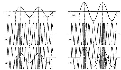
Fig. 2-1. The modulating waves in (A) and (B) are the same frequency,
but the amplitude of (A) is less than that of (B). The louder signal
(B) causes a greater frequency change in the modulated signal at (D),
shown by the increased bunching and spreading, than does the smaller
amplitude of (A) on the modulated signal at (C). In (E) and (F) the modulating
waves are superimposed on their respective modulated waves.
In the first Section we mentioned the frequency deviation of an FM signal and also how the amplitude and frequency of the audio modulating signal changed the degree of deviation and the repetition of this deviation. To understand the effects that a changing modulating signal has on a carrier being frequency modulated, it is best to use illustrative examples. The basic FM wave usually has the bunching up of its cycles at the positive half of the audio modulating signal and the spreading of its waveform in the negative half of the audio modulating signal. It is this bunching and spreading of the FM waveform that undergoes changes with respect to variations in the amplitude and frequency of the audio modulating signal.
Fig. 2-1 shows two FM signals modulated by the same audio frequency in each case but with the amplitude of the modulating signals different from each other. Parts (A) and (B) represent sinusoidal audio signals that are used to frequency modulate a carrier wave. Both are OI the same frequency, but signal B is of a louder tone than signal A as witnessed by the differences in amplitude. Wave C represents that FM wave modulated by the audio at (A), and wave D represents that FM wave modulated by the audio at (B). Comparing the two FM waves at (C) and (D), it is at once evident that an increase in loudness or audio level causes a greater frequency change (that is, deviation) of the modulated signals. In other words, the frequency deviation of wave D is greater than that of wave C. Upon further examination of these modulated waves, it will be noticed that when the modulating signal is positive (above its axis) then the frequency of the FM wave is increased. This is indicated by a bunching up of the wave at this point. Likewise when the audio signal is negative (below its axis) the frequency of the FM signal is decreased.
This is indicated by a spreading of the wave at this point. This was all indicated in Fig. 1-13 of Section 1, but it is even more clearly evident in parts (E) and (F) of Fig. 2-1, wherein the audio modulating signals A and B are respectively superimposed upon the FM waves C and D. To show how the frequency of the audio modulating signal deter mines the number of times a second that the deviation of the carrier takes place, let us refer to Fig. 2-2. The two audio signals A and B are of the same amplitude but different in frequency. For the same period of time, wave A undergoes two cycles of frequency change and wave B undergoes three cycles. This time equality is indicated by time T1 equaling time T2. Part (C) of Fig. 2-2 represents the FM wave that is modulated with the audio at (A) and part (D) represents the FM wave that is modulated with the audio at (B). If these two FM waves are examined, it will be seen that for the same period of time wave D undergoes a greater number of cycles of frequency changes than wave C. That is, the frequency deviation, which is determined by the amplitude of the modulating signal, changes through its full range more often in wave D than in wave C. This is due to the fact, as stated before, that the modulating signal of (B) is higher in frequency than that of (A).
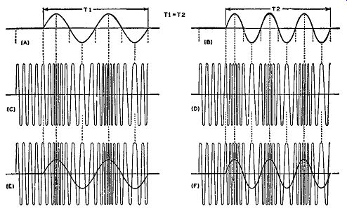
Fig. 2-2. The frequency of the modulating wave of (A) is less than that
of (B), the time intervals T1 and Ti being equal. Notice the two groups
of frequency changes in the modulated wave at (C) and the three in the
wave at (D), which occur in the same period of time. The modulating waves
are superimposed on their respective modulated carriers in (E) and (F).
Parts (E) and (F) of Fig. 2-2 show the audio signals superimposed upon the modulated signals in order to illustrate clearly that for the same period of time, the greater the frequency of the modulating signal, the greater the rate of change in FM deviation. The amplitudes of both audio signals are the same, and thus the amount of carrier frequency change or deviation is the same in each case. This is easily seen by comparing the points of maximum and minimum frequency in both FM waves and it will be seen that the points of closest bunching, as well as the points of greatest spacing, in each wave are equal to each other. However, since the frequencies of the audio modulating signals differ, with that at (B) greater than that at (A), the number of times per second that the cyclic frequency change takes place is different. The change of the modulated wave at (D) is seen to be more frequent than that at (C), indicating that the higher the audio frequency, for the same amplitude, the greater the number of times per second the deviation changes. Although technically accurate, the wave forms in both Fig. 2-1 and Fig. 2-2 have been exaggerated to provide a more vivid illustration.
FM Bandwidth and Sidebands
It was noted in Section 1 that in the a-m form of transmission the modulated wave (when at or under 100 percent modulation) consisted of three component waves. These three components were the carrier frequency and the upper and lower sidebands respectively.
In the FM form of transmission the modulated wave consists of the carrier frequency and numerous sideband components. In AM the frequency of the audio modulating signal determines the bandwidth.
Since 7500 cycles-per-second is the normal maximum amount of audio modulating frequency that can be used, the usual maximum band width in the a-m broadcast band is considered to be 15 kilocycles.
----
According to the FCC, modulation above 7.5 khz is permissible. however, if a station that modulates above 7.5 khz interferes with reception of signals from other stations, the interfering station has to install equipment or make adjustments to reduce this interference so that it is not objection able. Thus, in AM, 7.5 khz is considered as the normal maximum audio modulating frequency.
----
In FM the amplitude of the audio modulating signal is the chief factor in determining the amount of FM bandwidth. This was indicated in Fig. 2-1, where the difference in audio amplitude produced a different frequency change or deviation. This deviation may shift the frequency of the carrier by 50 khz, or even higher, according to the amplitude of the modulating signal. Since the allowable bandwidth in FM can be greater than that of the audio frequency spectrum, there is really no limit to the amount of audio frequencies that can be passed. Hence, in FM high fidelity can be easily attained. In deter mining the amount of deviation of the carrier, the amplitude of the modulating signal determines the effective bandwidth and also the number of effective FM sidebands.
The extent of the bandwidth, being dependent upon the variable factor of audio amplitude, is also a variable factor itself. The deviation in FM can vary by quite a large amount, and to compensate for the maximum amount of carrier frequency swing that can occur the FCC has established 75 khz as the peak deviation (that is, the maximum deviation on either side of the carrier). To this 75- khz deviation the FCC has added 25- khz guard bands making a total of 100 khz on either side of the carrier. The "guard bands" are included to insure against interaction between any two adjacent stations. For instance, without guard bands, if a station were somewhat off carrier frequency the shift might cause the bandwidth of the station to overlap that of the adjacent one. Consequently, the separation between adjacent channels in the FM broadcast band is 200 khz (100 khz on either side of the carrier). This 200- khz adjacent channel separation is for FM stations assigned to different coverage arec1.s. Adjacent channel stations that service the same area are separated by a minimum of 400 khz. The reason for this is primarily that the signals of stations covering the same area (as the New York City Metropolitan area) are quite strong, and there is probability of interference if there is any overlapping of the station bandwidths.
In AM the bandwidth is a much larger fraction of the carrier frequency than it is in FM For example, considering 1000 khz as the mean carrier frequency in the a-m band, the fraction of the 15- khz a-m bandwidth to this mean carrier frequency is: 15 khz/1000 khz= 0.015 or 1.5 percent of the carrier frequency. Considering the mean carrier frequency of the new FM band as being 100 mhz, the fraction of the FM bandwidth (150 khz or 0.150 mhz total) to this carrier frequency is 0.150/ 100 = 0.0015 or 0.15 of 1 percent. Examination of these relative percentages reveals why such a comparatively large bandwidth in FM is feasible, especially when it is such a small part of the carrier frequency.
The preceding Section stated that the a-m wave was a complex signal in that it contained various frequency components. The a-m wave and its component parts for 100 percent and 50 percent modulation were illustrated in Figs. 1-7 and 1-8, respectively. Besides the carrier, the other component parts of these modulated waves are known as the sidebands, and only two such sidebands (upper and lower) exist for each type of AM illustrated for sinusoidal modulation. In FM the situation is completely different. The FM wave is also a complex wave, but it contains numerous sideband components distributed equally on either side of the carrier frequency. The intelligence is contained in these FM sidebands as it is in AM with the difference that in FM the intelligence is distributed over a very wide spectrum of the sideband components. The amplitude of these side band components is not the same, as in AM, but varies considerably.
To prove that numerous sideband components of various amplitudes may exist in an FM signal for a single modulating frequency, higher mathematics would have to be used; this is beyond the scope of this guide. Although numerous sideband components do exist, the relative amplitudes of each determines whether or not they will be useful in the reproduction of the intelligence conveyed in them. In other words, the amplitude of a certain sideband component may be so small that it has negligible effect upon demodulation. This will become clearer if a spectral picture of the components of an FM signal is analyzed.
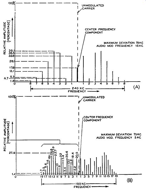
Fig. 2-3. Two spectral distributions of FM waves. The frequency of the
modulating signal in (A) is 15 khz and in (B) it is 5 khz. Note that
the relative amplitudes of the sidebands are often greater than the amplitude
of the center frequency component.
Two spectral distributions of FM waves are shown in Fig. 2-3. In both parts of this figure, the frequency of the unmodulated carrier is the same. The peak deviation involved is the same in either case, being 75 khz on either side of the carrier, even though the frequencies of the audio modulating signals differ. Since the deviation is the same in both cases, the amplitude of the audio is also the same. In part (A) of Fig. 2-3 the audio frequency involved is 15 khz, which is considered the maximum modulating frequency for high-fidelity FM The true amount of sideband components that exist are numerous, but the amplitudes of those past the 8th sideband are so small as to be ineffective in reproducing the sideband intelligence. In reality, there fore, there exist eight effective sideband pairs in the spectrum of part (A). Note that the amplitudes of the sideband pairs have no immediately apparent special order of increasing or decreasing in size. In fact, the amplitude of some of the sidebands may be greater than the center frequency component, which is the case for both spectra of Fig. 2-3. This contrasts with AM where the center frequency component is always greater in amplitude than its sidebands and equal to the amplitude of the unmodulated carrier. That is one of the reasons why FM is considered better than AM This will be expanded later.
As previously mentioned, the sidebands in FM are equally distributed on either side of the center frequency component. (The center frequency component is at the same frequency as the unmodulated carrier but always smaller in magnitude). This frequency distribution of sidebands is as follows: 1st sideband pair = center frequency + 1 X audio frequency 2d sideband pair = center frequency + 2 X audio frequency 3d sideband pair= center frequency+ 3 X audio frequency 4th sideband pair = center frequency + 4 X audio frequency and so on for as many effective sidebands as there are. Consequently, the first pair of sidebands in part (A) of Fig. 2-3 is found 15 khz on either side of the center frequency component. The second pair is found 2 X 15 khz or 30 khz on either side of the center frequency, the third pair 3 X 15 khz or 45 khz on either side, and so on. Therefore, the total distribution of the eight effective sidebands on one side of the center frequency in part (A) is equal to 8 X 15 or 120 khz. This means that the total effective bandwidth is equal to 240 khz.
Part (B) of Fig. 2-3 illustrates a similar situation where the modulating frequency is 5 khz. However, the number of effective sideband pairs in this case is greater and equal to 19. Since the sideband frequency distribution on either side of the center frequency is an integer multiple of the audio frequency, the effective bandwidth is 19 X 5 or 95 khz on one side of the center frequency. This means that the total effective bandwidth in part (B) is only 2 X 95 khz or 190 khz. This is 50 khz less than the bandwidth of the spectral distribution of part (A) of Fig. 2-3.
To indicate the relative amplitudes of the sidebands, they are shown to be some percentage of the amplitude of the unmodulated carrier, which is considered to be at 100 percent for maximum amplitude. The unmodulated carrier is drawn in dashed lines for the sake of clarity, but it really does not exist in the spectral distribution. In part (A) of Fig. 2-3, the center frequency component is seen to be only 17.8 percent of the unmodulated carrier. The first sideband pair is greater in magnitude than the center frequency, and it is 32.8 percent of the amplitude of the unmodulated carrier. The second sideband pair is only 4.66 percent of the unmodulated carrier. The amplitudes of the other sideband components vary accordingly, and their percentages are illustrated to the left of the spectrum.
In part (B) of Fig. 2-3, the relative percentage amplitudes are also illustrated to the left of the frequency spectrum.
Now that we have a fair understanding of FM spectrum distribution let us study the two spectra of Fig. 2-3 for comparison and try to formulate a general rule about spectrum distribution in FM in regard to deviation, bandwidth, and audio modulating frequency.
With the frequency deviation kept constant, the number of effective sidebands increases with a decrease in audio modulating frequency. However, the effective bandwidth does not increase with the increase in sidebands but rather decreases. This is evident from the two spectra of Fig. 2-3. In both cases the deviation is the same, being 75 khz. In part (B) the audio frequency is 5 khz, and the number of effective sideband pairs 19, but the effective bandwidth is only 190 khz. If the audio frequency is 3120 cycles, the number of effective sideband pairs would be 29, but the effective bandwidth would only be 181 khz.
The actual determination of the amplitude of the sidebands employs higher mathematics, namely Bessel Functions, and is beyond the scope of this guide.
Consequently, a general rule can be formed regarding FM spectrum distribution. With the frequency deviation assumed constant, the greatest bandwidth (spectrum distribution) is attained when the audio modulating frequency is at its highest value. As this audio frequency is lowered (keeping the deviation still constant), the effective bandwidth decreases, but the number of effective sidebands increase. However, no matter how low the audio frequency is made and no matter how many effective sidebands do appear, the effective bandwidth can never be reduced below the frequency deviation on either side of the carrier. If twice the audio modulation frequency happens to be higher than this peak-to-peak deviation swing, then the effective bandwidth cannot be less than twice this audio frequency. Therefore, with a deviation frequency of 75 khz on one side of the carrier, the effective bandwidth can never be less than 150 khz since the audio frequency cannot exceed the deviation.
After a spectrum analysis, the question invariably arises as to what would happen if the frequency deviation were not kept constant, if the audio frequency were kept constant and the deviation varied. The answer to this is relatively simple if one fully understands the fore-going analysis.
Let us assume the audio frequency to be constant at 10 khz and the peak deviation varied from 60 khz to 30 khz. Where the peak deviation is 60 khz, the number of effective sidebands that appear in the frequency spectrum is 18 (9 sideband pairs) and the effective bandwidth is then equal to 18 X 10 khz or 180 khz. Where the peak deviation is 30 khz, the number of effective sidebands that appear is only 12 (6 sideband pairs) and the effective bandwidth in this instance is only 12 X 10 khz or 120 khz. Consequently, in this type of spectrum distribution decreasing the frequency deviation while keeping the audio frequency constant decreases both the number of effective sidebands and the effective bandwidth.
Both where the deviation is held constant and the audio frequency varied and where the audio is held constant and the deviation varied, a fundamental relation exists between the frequency deviation and the audio modulating frequency. This relation is known as the modulation index or deviation ratio and will be discussed in greater detail later on.
To emphasize the fact that some sidebands of an FM wave can be (and often are) greater in amplitude than the center frequency component, a breakdown of a typical FM wave will be illustrated. In part (A) of Fig. 2-4 is shown a typical FM wave together with the unmodulated carrier signal. The unmodulated carrier frequency is designated as fa and the audio modulating frequency as fA.- If the amplitude of the audio signal is such that a peak deviation (designated as fD) of 30 khz appears for an audio frequency of 15 khz, the number of effective sideband pairs is only four. These are illustrated together with the FM wave and the spectrum distribution in Fig. 2-4.
The maximum instantaneous frequency is equal to the carrier frequency plus the frequency deviation. In respect to what was discussed in Section 1 this takes place at the maximum point of the positive half cycle of audio. The minimum value of the instantaneous frequency of the FM wave is equal to the carrier frequency less the frequency of deviation. This takes place at the maximum point of the negative half cycle of audio. These maximum and minimum frequency points are indicated in the FM wave of Fig. 2-4. If the respective amplitudes of the carrier and center frequency component are examined, it will be noted that, although they are equal in frequency, the amplitude of the center frequency is much less than that of the carrier. In fact in the case shown here, where the deviation is equal to 30 khz and the audio equal to 15 khz, the amplitude of the center frequency component (B) is equal to 22.4 percent of the unmodulated carrier amplitude. This is very different from the a-m case where the amplitude of the center frequency component is equal to that of the carrier.
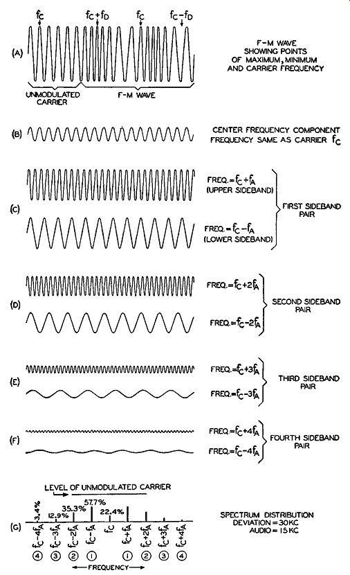
Fig. 2-4. Analysis of an FM wave with respect to its sidebands and center
frequency component.
If the first sideband pair (C) of signals is examined, it is noted that their amplitudes are much greater than that of the center frequency component. The same is true of the second (D) sideband components.
However, the third (E) and fourth (F) sideband pairs are smaller in amplitude than the center frequency component, part (B). The relative frequencies of the sideband components are indicated next to their waveforms. The spectrum distribution of the components parts of the FM wave is illustrated in part (G) of Fig. 2-4.
Since the center frequency component of the FM wave does not contain any of the intelligence (that is, audio modulating signal), then the smaller its amplitude, the less power wasted. In AM, half the power of modulation (for 100 percent modulation) is invested in the center frequency component, which is equal in amplitude to that of the carrier, and the power unavoidably contained in it is wasted so far as demodulation at the receiver is concerned. Therefore, the audio modulating equipment for high level AM has to be high powered in order that the sidebands contain a sufficient amount of power for proper demodulation. In FM the situation is different, especially where more than three pairs of sidebands are present. Most of the power in FM is distributed in its sidebands, while the center frequency component of the FM wave contains a relatively small part of the transmitted power. In AM, modulation increases the radiated power, whereas in FM the power remains constant.
This is one of the important reasons why FM transmitters are so much cheaper to operate than a-m transmitters. There is greater power efficiency in FM than in AM Since FM does not require high powered equipment, receiving type tubes can be used for its modulating and speech equipment.
A similar analysis to that given in this section exists for p.m. Because the analysis is basically very much alike, only the one for FM was studied.
Percentage of Modulation
An interesting highlight of FM is the percentage of modulation. In AM the percentage of modulation is a direct relation between the audio power and the power of the unmodulated carrier. In this respect the greater the percentage of modulation (up to 100 percent), the greater the audio power output from the receiver. If the percentage of modulation is increased beyond 100 percent (overmodulation), it means that the audio power at the transmitter is greater than the r-f carrier power. If an overmodulated a-m wave is transmitted and picked up by a receiver, distortion results in the receiver output be cause overmodulation causes distortion of the a-m transmitted signal.
(See Fig.1-5 Section 1). A somewhat different situation exists for FM in regard to the percentage of modulation. Reference to the percentage of modulation in FM as is done in AM would presuppose a condition practically impossible to attain. For instance, in AM the power or level of audio modulation with respect to that of the carrier determines the percentage of modulation. When the power of the audio signal equals that of the carrier, 100 percent modulation exists. In FM the level of the audio modulating signal determines the frequency deviation of the carrier. In this respect then, what would be a good method of determining percentage of modulation for FM? Since the level of the audio signal determines the frequency deviation for FM, it should follow that the relation between the frequency deviation of the carrier and the frequency of the carrier would be a good method of determining percentage of modulation for FM This follows somewhat similar lines for percentage of modulation in AM However, if this definition for percentage of modulation were to hold true for FM, the peak frequency deviation would have to equal half of the carrier frequency for 100 percent modulation. For a carrier frequency of 100 mhz the peak deviation frequency would have to be equal to 50 mhz. This is known to be definitely out of the question for more than one reason.
First of all, the level of the audio would have to be quite high and the level of the carrier quite low. Secondly, the deviation necessary would cover too wide a frequency range; it would be completely outside the FM band.
Since such a definition is not realizable, percentage of modulation in FM is defined in another way. It is based upon the maximum available deviation incorporated in the individual transmitter. If an FM transmitter has provisions so that the audio level will never produce deviations in the carrier greater than a certain amount, then for that amount the transmitter will be working at 100 percent modulation. Since the maximum deviation as set up by the FCC cannot be greater than 75 khz for commercial broadcasting, then 100 percent modulation for FM can never exceed a frequency deviation of 75 khz.
This definitely places a limit on the level of audio modulating signal.
Whenever the audio level increases to a point where it produces a frequency deviation greater than 75 khz, overmodulation for FM is said to exist. The audio level in FM is seen to exercise a different type of control, so far as percentage of modulation is concerned, than it does in AM Briefly, then, 100 percent modulation for FM becomes equivalent to the maximum allowable frequency deviation.
Modulation Index - Deviation Ratio
Two of the most important factors in FM broadcasting are the deviation swing and audio modulating signal. Associations between these two quantities enable us to bring out some very important relations about FM The basic relationship between these two quantities is the ratio of the peak frequency deviation swing to the audio modulating frequency. This ratio, as mentioned above, is known as the modulation index or deviation ratio. One of the most common symbolic methods of representing this ratio 1s by the letter M. Some texts use the Greek letter beta, β, but in this guide we will use the former. This ratio is very important in establishing the number of effective side bands and the effective bandwidth.
TABLE 1
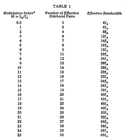
• All the M's that are less than 0.5 have only one pair of effective side bands and their effective bandwidths are all equal to 2fA.
Let us examine this ratio and see what importance it holds. Calling the peak deviation frequency fD and the audio modulating frequency f.a, the index ratio is given by the following:
Modulation index: M = ~:
When it is realized that the level of the audio modulating signal determines the amount of deviation and that the audio frequency is also relevant to the value of M (the frequency of the audio is the denominator in the foregoing expression for M), the importance of the modulating signal becomes apparent. It is known that the higher the level of the audio signal, the greater the deviation swing and, consequently, the greater the modulation index M (for a given audio frequency). This ratio M is important in that it helps determine the number of effective sidebands and the effective bandwidth.
The chart in Table 1 will help determine these factors, once the peak deviation swing, fD, and the audio frequency, fA, are known. The first column is for the modulation index, where M equals the previously explained ratio. The second column depicts the number of effective sideband pairs. With the multitude of sidebands occurring in FM, some limit has to be set to define what is no longer an effective sideband. The amplitudes of the sidebands in FM vary considerably. Some are greater in amplitude than others. The second side band pair may be so small as to be non-effective, while the third and fourth may be appreciably large - even larger than the center frequency component. However, as we proceed farther away from the center frequency component a point will be reached after which the sideband components will all become very small. The point where the amplitudes of the sidebands become appreciably less than one percent of the amplitude of the carrier is the determining margin of effective bandwidth. In other words, the number of sidebands between this point and the center frequency component of the FM wave is the number of effective sideband pairs (the sidebands appear equally on both sides of the center frequency component). These effective side band pairs appear in the second column of Table 1. In the third column the effective bandwidth is included. This effective bandwidth is based upon the number of effective sideband pairs included in the second column. To find the effective bandwidth, the number of effective side bands on both sides of the center frequency component is multiplied by the frequency of the audio modulating signal. Using Table 1 is a simple procedure. The following example will indicate the simplicity of its use.
If the peak deviation frequency as caused by the amplitude of a 5- khz audio modulating signal is equal to 35 khz, the modulation index is 35 /5 or 7. Looking down the first column of Table 1 to the modulation index of 7 it is found from the second column, that the number of effective sideband pairs is 11 and the effective bandwidth from the third column is 22fA- Since the audio modulating frequency involved is 5 khz, the total effective bandwidth is 22 X 5 or 110 khz. This does not necessarily mean that in all cases where Mis equal to 7 the bandwidth is going to equal 110 khz. Only the number of effective sideband pairs remains the same for the same value of M. For instance, if the peak deviation frequency was 70 khz and the audio frequency 10 khz, the index M would still be 7 and the number of effective sideband pairs still 11. However, the bandwidth in this latter case is equal to 22f A or 22 X 10 khz, or 220 khz, which is exactly double the previous bandwidth.
Even when the modulation index happens to be some fractional number lying between the numbers in the first column, the effective bandwidth and number of sideband pairs can be easily determined from the table. For instance, if M turns out to be 9 ¼, then the modulation index of nine should be used. If M is 9 ¾, then the modulation index of 10 should be used. In other words, whichever number the fractional M is nearer is the one used.
If the modulation index M is less than ½, the number of effective sideband pairs is only one, which is similar to AM (This is the basis upon which the Armstrong transmitter was designed.) Since one pair of effective sidebands always exists when Mis less than ½, the effective bandwidth can never be less than two times the audio frequency (2fA). Consequently, when the audio modulating signal is higher in frequency than the peak deviation frequency, the effective bandwidth can never be less than twice the audio frequency. As the modulation index M increases, but the deviation remains constant, the number of sideband pairs also increases, but the effective bandwidth decreases as previously mentioned. However, no matter how much M increases, which means no matter how high f O becomes and how low f A becomes, the bandwidth can never be less than the peak-to-peak deviation of the carrier frequency. In other words, the effective bandwidth can never be less than twice the audio frequency or the peak-to-peak deviation swing, whichever is greater.
So far we have dealt primarily with the modulation index with respect to the amount of frequency deviation and have said nothing about phase deviation. In some transmitters the oscillator is directly frequency modulated, and when this type of modulation occurs, we invariably refer to the frequency deviation. In indirect FM transmitters, where the oscillator signal is initially varied in phase about its relative phase angle, we talk in terms of the amount of phase deviation. In Section 1 we showed that a shift in phase is equivalent to a change in frequency and vice versa. Consequently, when talking in terms of frequency deviation, we can also refer to the equivalent amount of phase deviation. Likewise, when talking about phase deviation we can also refer to its equivalent in frequency deviation. however, if the transmitter is one of direct FM, usually only frequency deviation will be referred to, but in indirect FM transmitters phase deviation is a common term. The amount of equivalent frequency deviation is also mentioned in reference to indirect FM transmitters, because it is becoming accepted practice to talk in general terms of frequency deviation.
Once the modulation index M is known, it is a simple process to find the amount of equivalent phase shift. A circle, or one cyclic change of alternating signal, is said to contain 360 degrees or 2 pi radians, where 1r is a numerical figure equal to 3.14. Therefore, one radian is said to contain 360/2 π degrees or 360° /6.28 or 57.3°. Since the modulation index M as discussed is given a value on the basis of cyclic changes, if we multiply the modulation index M by 57.3 degrees, we will get the equivalent phase shift in degrees. For instance for a modulation index of 7 the equivalent phase shift is equal to 7 X 57.3 = 401.1 . This phase shift is known as the phase deviation. If ascertain indirect FM transmitter is found to have a peak phase shift at the output of its oscillator-modulator system of 25 degrees for an audio frequency of 50 cycles, it is often desired to know what the equivalent peak frequency deviation is. Since the peak phase deviation, call it PD, is equal to M times 57.3 and since M is equal to fD/fA (the peak deviation frequency fD divided by the audio modulating frequency fA) then we have the relation:
PD=MX57.3° or PD=~ X 57.3° solving for fD we find that f
_ PD X fA D - 57.3°
For the problem under discussion PD equals 25 degrees and f A equals 50 cycles, therefore the equivalent peak frequency deviation is equal to:
25° X 50 fD = 57
_ 30
= 21.8 cycles
From this analysis we see that we can talk in terms of phase deviation as well as frequency deviation.
Interference Between Signals
When FM was introduced to the public its biggest drawing card was its successful method of minimizing interference disturbances usually found with AM Many of us have some basic knowledge of the concept that in FM receivers, amplitude limiters or other means are employed to reduce greatly the effects of amplitude variations on an FM signal. The type of interference we are concerned with at the moment is that between two of the same types of modulated signals.
Interference between a-m waves is quite well known. Some of this interference is due to image frequency effects which are definitely undesirable in any receiver. It is the purpose of this section to indicate why such types of interference and others are less likely to occur in FM than in AM So far as interference between two a-m waves is concerned, let us consider two forms. First, there is interference between two stations that operate on the same or near the same frequency but are, presumably, in different service areas. Secondly, there is the interference between two stations of different frequency, when one is the image frequency of the other. In regard to the former case, if the amplitude of the signal from the station considered to be the interfering one is only 1 percent of the a-m wave from the station being interfered with, the interfering effect will be noticeable. In other words, if an interfering signal is of the same frequency as an other signal (or differs so slightly in frequency as to be passed by the selective circuits in the input to the receiver) and if its amplitude is only one hundredth as great as that of desired signal, then the interference will be perceptible in the output of the receiver. When image frequencies appear, the same situation prevails in regard to the amplitude of the interfering signal with respect to that of the desired signal. To state it in another manner, the amplitude of the desired a-m signal has to be at least one hundred times as great as the amplitude of the interfering signal, no matter what its source, in order that the interfering signal have little or no effect.
If the interfering signal is of the same frequency as the desired signal, the amplitude of the desired signal as it passes through the receiver is changed in accordance with the amplitude variations of the interfering signal. Consequently, the output of the receiver contains the intelligence of both the desired signal and the undesired signal.
The weaker the undesired signal, the weaker is the interference output. However, as long as there exists a ratio between the amplitude of the desired and undesired signals that is greater than roughly 100 to 1, then interference in the output of the receiver will be undetected.
When the interfering signal differs so slightly from the desired signal that the selective circuits are broad enough to pass it, then besides interference between the intelligence of the two signals in the output of the receiver, a heterodyne squeal will probably be heard. This squeal is due to the slight difference in frequency between the interfering and desired signal. In other words, the interfering signal varies the amplitude of the desired signal in accordance with its varying amplitude, producing a new varying amplitude. This varying amplitude occurs at a frequency that is the difference between the two signals. If this difference is within the audio range, it will appear in the output as a heterodyne squeal. This latter condition of interference is quite complicated, inasmuch as three different types of output are really detected, the intelligence of both the desired signal and the interfering signal and the heterodyne squeal. Consequently, as far as AM is concerned, the signal to noise ratio or the ratio of desired to undesired signal has to be greater than 100 to 1 for interference to be undetected in the output of a receiver.
The FM situation is completely different. If the ratio in FM of the desired signal to an undesired signal on an adjacent channel is as small as 2 to 1, interference will not affect the output as far as the listener is concerned. Though this has been definitely proved by field tests as well as by mathematical analysis, the details are beyond the scope of this guide. It is sufficient to state that if the modulation index of the desired signal is high, the chances of interference become reduced. There exists a limitation in the amount of angular variation between the desired and interfering signal such that no matter what the phase variation of the interfering signal, the resultant signal from the interference can never have a deviation ratio (modulation index) greater than ½. Therefore, if the modulation index of the desired signal is made greater than this maximum resultant signal's modulation index of ½, the chances for interference will be greatly reduced.
Two things are basic to the proper discrimination against interfering signals in FM If the amplitude of the desired FM signal is at least twice as great as the amplitude of the interfering signal, the interfering signal will have practically no effect. In addition, the modulation index should be higher than ½, and the higher the better.
Even though these standards may be met in practice, it is possible that under some peculiar circumstances, such as a receiver located between two transmitters and perhaps at the limit of the range of transmission of both stations, or a terrain of a special nature, this desired ratio of 2:1 will not prevail. Under these conditions both signals will be heard.
This will be discussed in Section 5.
So far as the receiver itself is concerned, nothing can be done to alleviate the situation, because no amount of alignment or readjustment within the receiver proper can in any way raise the level of the desired signal and reduce the level of the undesired signal. The one possible solution that remains is use of a directional antenna, so that a stronger signal is secured from the desired station.
QUESTIONS
SECTION 2
2-1. a. If the amplitude, or strength, of the audio modulating signal of an FM wave is increased (assuming a constant audio frequency), what happens to the frequency deviation? b. How does this change in audio signal level affect the appearance of the FM wave?
2- 2, a. If the frequency of an audio modulating signal is increased (assuming no change in its amplitude), what happens to the amount of frequency deviation? What happens to the rate of frequency deviation? b. For the same period of time how does this change in audio frequency affect the appearance of the FM wave, still assuming no change in amplitude of the audio signal?
2-3. What is the chief factor that determines the effective bandwidth in a-m broadcasting? In FM broadcasting?
2-4. What purpose does the 25-khz "guard band" serve?
2-5. What is the minimum adjacent channel separation for FM stations assigned to the same coverage area? Why this amount?
2-6. Why is such a large bandwidth allowable in FM as compared with that in AM?
2-7. a. Are FM signals limited to two sidebands? b. In an a-m signal, the center frequency component is always much greater in amplitude than the sidebands. Is this also true of the center frequency component of an FM signal? Explain. c. Is there any particular order in which the amplitudes of the side bands of an FM signal increase or decrease? d. What determines whether a sideband of an FM signal is considered effective?
2-8. a. What is a sideband pair? b. If an audio modulating frequency is equal to 7 khz and if the center frequency of an FM signal is equal to 96.1 mhz, what are the frequencies of the fifth sideband pair? c. If the FM wave of part (b) is assumed to have only 14 effective sideband pairs, what is its effective bandwidth?
2-9. a. If the audio modulating frequency of one FM signal is higher than another, which FM signal has the greater number of effective sidebands, assuming that the strength of each modulating signal is the same? b. Which signal has the greater effective bandwidth?
2-10. Taking into account the amount of frequency deviation and the audio modulating frequency, what is the minimum limit of the effective bandwidth of an FM signal?
2-11. a. If the amplitude of the audio modulating signal of one FM wave is higher than another, which FM signal has the greater number of effective sidebands, assuming that the audio modulating frequency is the same for both? b. Which signal has the greater bandwidth?
2-12. If the amplitude of a 10- khz audio signal is such that it produces a peak-to-peak frequency swing of 40 khz in frequency modulating an r-f carrier of 100 mhz, then: a. What is the maximum instantaneous frequency of the FM wave? b. What is the minimum instantaneous frequency of the FM wave?
2-13. Where is most of the power found in an a-m signal? Compare this situation with that of an FM signal?
2-14. a. If we were to interpret percentage of modulation of an FM signal (in terms of frequency deviation and carrier frequency) in a similar manner to the way it is defined in an a-m signal, what would be the equivalent of 100-percent modulation in FM? b. What represents 100-percent modulation in FM broadcasting to day?
2-15. a. Define the modulation index. b. What is another name for the modulation index?
2-16. Explain how both the amplitude and frequency of the audio modulating signal are represented by the modulation index.
2-17. a. If an audio signal is equal to 10 khz and the peak-to-peak deviation of an FM signal is equal to 100 khz, what is the modulation index? What is the effective bandwidth of the FM signal? Hint: Use Table 1. b. If a 100-mhz carrier is frequency modulated by a 7-khz audio signal such that the FM signal has a maximum instantaneous frequency of 100.056 mhz, what will be the effective bandwidth of the FM signal? Hint: Use Table 1. c. If the audio modulating signal of an FM wave is equal to 8 khz, the carrier frequency equal to 90 mhz, and the effective bandwidth equal to 144 khz, what will be the minimum instantaneous frequency of the FM signal? Hint: First find the modulation index. d. If the audio modulating frequency is 15 khz and the peak frequency deviation of an FM signal equals 5 khz, what is the effective band width of the FM signal?
2-18. a. If at an audio modulating frequency of 100 cycles the peak-to-peak frequency deviation of an FM wave is equal to 80 khz, what is the equivalent peak phase deviation? b. If the peak phase deviation of an FM signal is equal to 520 degrees and the audio modulating frequency equals 5 khz, what is the effective bandwidth of the FM signal?
2-19. a. In a-m how much greater does the amplitude of a desired signal have to be than that of an undesired signal to prevent interference from the latter? b. Under most circumstances how strong must a desired FM signal be to just eliminate noticeable interference from an undesired signal?