With the transmitter tuned up for maximum output from the r-f final amplifier, the object now is to get the energy into the antenna with the least amount of loss, and to tune the antenna for most effective radiation of the signal. Factors which affect the signal are: antenna resonance at the operating frequency, feed-line losses, and matching the feeder impedance to the antenna.
The most important antenna factor is antenna resonance. Any piece of wire, because of the inductance and capacitance distributed along its length, is resonant at some frequency. It is a resonant circuit like a coil and capacitor, and, theoretically, looks something like Fig. 6-1.
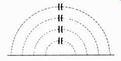
Fig. 6-1. Any piece of wire has inductance and distributed capacitance; therefore,
any wire will resonate at some frequency.
Its length is closely related to the resonant frequency. A piece of wire 80 meters, or 262.5 feet, long will resonate at about 80 meters (3.75 MHz). The wire is said to be one wavelength long. It will also resonate at one-half wavelength long, and it then becomes a half wave dipole.
The mechanical length of a half-wave dipole is slightly shorter than its electrical length. A factor (X) is involved in the formula. K is affected by the ratio of wire length to diameter of wire, and is theoretically 1 for an infinitely long wire of infinitesimally thin diameter.
The factor K is .95 for most practical antennas for frequencies up to about 30 MHz, considering the usual wire size and length and the fact that it is not truly in free space (infinitely high). Taking into account K = .95, and converting to feet, the usual formula for a half-wave dipole is:
Length (in feet) = 468/f
where,
f is the frequency in MHz.
A piece of information important in tuning an antenna is what it looks like to the end of the feed line. This is the factor of radiation resistance. The very center of an ideal half-wave dipole (one with a factor of K = 1 ) at resonance is equivalent to pure resistance of 73 ohms. That is, if it were replaced by a noninductive resistance of 73 ohms, the end of the feeder would not know the difference. At the center of an antenna the reactances (C and L) exactly cancel and the net effect is zero reactance or a pure resistance. The impedance (a combination of resistance and reactance) increases farther out from center, and is theoretically infinite at the ends. Maximum current and minimum impedance occur at the center; zero current and maximum impedance is at the ends. An antenna is affected by many factors: length of wire to diameter; height above ground; capacitance effect of nearby metal objects, reflectors and directors; etc. The center impedance of a 3-element beam is more like 15 ohms, for example, and the center of a half-wave dipole fairly clear above ground is usually around 72 ohms. What is important to tuning an antenna is to know that the center looks like a pure resistance, whatever its value may be.
The point to remember is that the R of the center of the antenna is the load on the transmitter, whether it is applied through a feeder or a combination of feeder and some transformer device.
TUNING THE ANTENNA
If you can get to the center of the antenna there are two methods of measuring for resonance. Each uses inexpensive equipment, the GDO (grid-dip oscillator) and the impedance bridge.
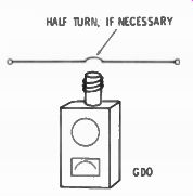
Fig. 6-2. An AC operated or sensitive battery-powered grid-dip oscillator
will measure resonance when coupled to the center of a half-wave dipole.
Couple the coil of a GDO to the closed center of the antenna (Fig. 6-2) and tune the GDO for a dip in the meter. For least effect of the GDO on the resonance of the antenna, the coupling should be as loose as possible and still be able to discern a dip in the meter. The best type of GDO out in the field away from AC power is a battery operated GDO using transistors or a tunnel diode. After getting the dip bring the GDO into the shack and check the frequency with your receiver. The accuracy of calibration of the usual GDO is not good enough for exact frequency measurement.
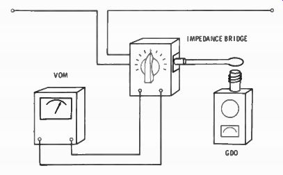
Fig. 6-3. Driving an impedance bridge with a GDO will give you antenna resonance
and impedance at the center.
Method two uses a GDO and an impedance bridge (Fig. 6-3). The X (unknown) terminals of the bridge connect to the center of the antenna. The GDO is the signal source of the bridge. The output of a battery-operated GDO is pretty low, so it takes a very sensitive meter in the bridge circuit for an indicator. A 50-uA meter should be used.
Adjust both the GDO and the bridge impedance arm for a zero reading on the indicating meter of the bridge. When the meter reads zero,
the GDO is at the resonant frequency and the bridge will read the actual impedance of the center of the antenna. If no zero can be obtained it means you are not at the exact electrical center of the antenna. You may be physically, but the capacitance effects of nearby metal objects to the end of an antenna will shift the electrical center.
To find the electrical center, take a plier in your hand and touch along the antenna wire on each side of the feed point and watch the meters. Touching the antenna will cause both meters to jump a little.
When you have touched a point on the antenna where neither meter is affected, you have found the electrical center. You can move the center closer to the feed point in the manner in which you trim your antenna for resonance to the operating frequency. If the electrical center is found to be to the right of the feed point, add wire to the right end if the measured frequency is too high, or cut wire from the left end if the measured frequency is too low. If the electrical center is to the left of the feed point, add wire to the left if the antenna is too short, or cut wire from the right if too long.
To accomplish a feed-line condition with no standing waves on the feeder, the feeder must connect to the exact electrical center.
However, a small amount of reactance by being slightly off center will not have too much effect, and is usually not worth correcting.
The real problem in measuring antenna resonance is a physical one, how to get up there to the center of the antenna. High-frequency antennas and beams mounted on a roof are sometimes within reach.
Long-wire dipoles for the lower frequencies are strung between poles or similar structures and just cannot be reached easily. The answer is to do your measuring at the lower end of a feeder-of a half-wave feeder, that is.
THE HALF-WAVE FEEDER
A feeder of any type, which is exactly one-half wavelength long, will reflect the same load impedance to the transmitter as it sees at the antenna. When a half-wave feeder is connected to the feed point of an antenna, the radiation resistance of the antenna at resonance will also appear at the input end of the feeder. Therefore, the same measurements can be made to the antenna (via a feeder) in the shack.
The characteristic impedance of the feeder is not important. It is also not necessary that the feeder match the antenna at the feed point. It is only important that the feeder be exactly one-half wave length long electrically.
Coupling a GDO alone to the end of the feeder will not indicate antenna resonance. You will get a dip in the meter, but the resonance shown in the GDO will include any reactance in the feeder in case it is not an exact half wave in length. The best method of making a measurement is to use the number-two method mentioned earlier for measuring at the antenna, use a bridge and a GDO (or signal generator or even the transmitter vfo). The setup is shown in ...
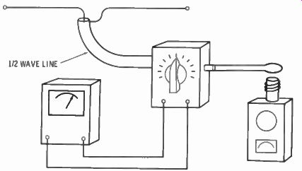
Fig. 6-4. Measurement of antenna resonance and impedance can be made from
the shack with a half-wave feed line coupling your test equipment to the antenna.
... Fig. 6-4. There will be a slight amount of error resulting from the use of a coupling loop at the input of the bridge because the reactance of the loop affects the frequency of the GDO. It can be eliminated by injecting a signal from a signal generator or your transmitter vfo and listening for the beat in the headphones plugged into the GDO, or by using a signal source such as a signal generator whose output cable is terminated with a resistor. Most signal generators worthy of the name have built-in terminations of 50 or 75 ohms.
The direct connection to the bridge eliminates the coupling loop.
Set the GDO to the operating frequency (the frequency for which the feed line has been cut). Turn the bridge control arm for a zero reading on the indicating meter of the bridge, or the VOM connected to it. If the indicator reads zero, the antenna is resonant at that frequency, and the center feed-point impedance is the impedance shown on the bridge. If the bridge-balance indicator cannot be zeroed, there is reactance at the feed point to the antenna, meaning either the antenna is not exactly resonant or the feed point is not at the electrical center. If a perfect balance is not obtained, readjust the GDO for the best dip in the GDO meter. The new frequency reading will indicate the direction in frequency the antenna is off. From then on it is a matter of cut and try on the antenna until operating resonance is reached. If. with the antenna at resonance and a perfect balance in the bridge (indicator at zero) the bridge impedance shown is not the same as the rated characteristic impedance of the feed line, there is a mismatch between feeder and antenna. The antenna is at resonance but the feed point is not a perfect match to the feed line. This may or may not be important, depending on how far off the mismatch is, and how long the feed line is. Power loss in the feeder will be a combination of its construction, effect due to an SWR (standing-wave ratio) other than 1:1, and its length. Table 6-1 lists popular coaxial cables for feeders and important characteristics, including the velocity factor which will be discussed shortly.
The impedance bridge used in this test is the one described in the next section. A 50-/uA meter movement gives about a one-third scale reading in the unbalanced condition when used with a GDO whose oscillator is a 6C4 tube powered from the 120-volt AC line. The author's portable GDO did not have sufficient oscillator power to operate the balance indicator.
HOW TO CUT A HALF-WAVE LINE
If you purchase brand-new, good-quality feed line (coax cable, for instance), be sure a recognized manufacturer's name and type number appears imprinted on the cable at intervals. Your choice of cable will depend on the amount of power you expect to handle and how much you can afford to spend to keep losses down. First determine how many feet you will need from Table 6-1. Use the velocity factor shown in the table in the following formula for length needed, and add a few feet for error and trimming:
Length in feet/492 = velocity factor f in MHz
This formula is set up as a ratio for easy slide-rule use. A half-wave feed line is open at both ends. Since it is difficult to couple a GDO to an open-ended feed line, short one end and measure it as though it were a quarter-wave long, but at half the frequency. Skin back one end and connect the inner conductor to the outside braid, and form a small loop, about the size of the GDO coils. Measure the exact physical length and calculate what the resonant frequency should be using the following ratio:
Length in feet _ V
* 246 J
where, V equals velocity factor, f equals frequency in MHz.
This ratio is based on the formula for a quarter-wave stub, and the figure for frequency used is one-half the frequency to which you want to cut the half-wave line. Now couple the GDO (tuned for half the desired frequency) to the loop and adjust the tuning dial for a dip in the indicating meter. It should be close to the frequency calculated based on its length and published V (velocity factor). If the frequency does not agree and you have used a non-branded and un marked cable, then suspect a difference in the velocity factor. Should you find this to be true, then solve for V in the foregoing ratio, and use the new figure for V to calculate the length of cable you will need for the frequency at which it is to operate. Cut the cable so it is only a few inches longer than desired.
Turn on your receiver and tune it to the middle of the band for which you want the half-wave cable. Couple the GDO to the loop on the cable and listen for its harmonic on the receiver (remember, the GDO is measuring at half the frequency). Cut off an inch at a time from the far, open end of the cable and re-dip the GDO until you hear the harmonic and see the dip at the same time. The feeder is now a half-wave line in the band you want. The results are the same whether the cable is stretched out or coiled up while making the frequency measurement.
An impedance bridge may also be used to measure a feed line for a half-wave length. Short the far end of the line and connect the open end to the X terminals of the bridge. Place the balance control at zero. Adjust the GDO used to drive the bridge for a zero balance on the bridge indicating meter. The line is a half-wave long at the indicated frequency. The measurement should agree with the formula:
L in feet 492 V
or the ratio for a slide rule is; L in feet _ V "492 T
Since a half-wave line reflects the same impedance at one end of the line as the other, a short at one end will measure zero impedance at the other. The hookup is shown in Fig. 6-5.
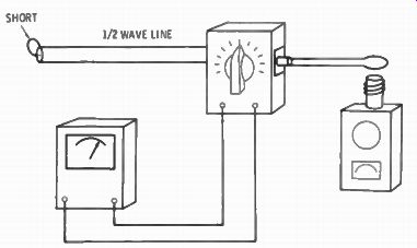
Fig. 6-5. A GDO and impedance bridge may be used to measure for a half-wave
line length. With a short at the end of the line and zero setting on the bridge,
the GDO will read the frequency when the indicator meter is at null.
While the line is set up for measurement for length and velocity factor you should make another check, and that is for characteristic impedance. This is particularly important on unbranded cable or on open-wire lines that you have made yourself. The hookup for this test is the same as in Fig. 6-5 and employs the impedance bridge and GDO. Instead of shorting the other end of the line, connect a carbon resistor whose value is that of the supposed characteristic impedance of the line between the two conductors. With the impedance-bridge control arm set at the value of the characteristic impedance, the balance meter should read zero. Furthermore, the meter should remain at zero with changes in frequency on the GDO. Should the meter not remain at zero with frequency changes, the characteristic impedance of the line is something other than the resistor value used at the end of the line. Substitute other values of resistors until there is no change. The final resistor value is the characteristic impedance of the line. The line can be any length for this test. With each change in resistor be sure to reset the balance arm on the impedance bridge to the same value as the resistor used.
MEASURING ANTENNA IMPEDANCE
With the half-wave feeder, GDO and impedance bridge, you are in a position to make a check of the impedance of the antenna at the center. This assumes that the antenna has been adjusted for resonance at the operating frequency.
The hookup is as shown in Fig. 6-4. Adjust the GDO to the frequency of the antenna and couple it to the input of the impedance
bridge. Adjust the balancing arm of the impedance bridge for a zero reading on the balance indicator. Since a half-wave feed line reflects the same impedance it sees at the far end, the impedance value indicated on the balance arm of the impedance bridge is the impedance of the antenna where the feeder connects to it. If it is the same as the characteristic impedance of the feeder you are matched, and any length of the same feeder, either longer or shorter than the half-wave length, may be used. However, if coaxial feed line is used you should correct the unbalance between the use of an unbalanced line to the balanced feed point on the antenna. This is corrected by using a 1:1 balun transformer at the antenna or by using a "gamma" matching device.
A word of caution on using the impedance bridge. Do not attempt to use the transmitter as the signal source of the impedance bridge.
The components of the bridge have limited power-handling capability, and if more than about 4 watts are used to drive the bridge, the components will bum out.
ABOUT SWR
If the above hookup shows a difference in impedance between the antenna and the characteristic impedance of the line, the mis match will result in standing waves on the line during transmission if it is not corrected. The extent of the standing waves is measured in terms of the ratio between the forward wave in the line and the portion returning, or reflected, back into the line as a result of the mismatch. Knowing the impedance of the feed point on the antenna and the characteristic impedance of the line, the SWR (standing wave ratio) is:
SWR = Z-A/Z_L
….where,
Z_A is measured impedance of the antenna,
Z_L is the characteristic impedance of the line.
THE VALUE OF A LOW SWR
While the insulating material used inside the coaxial cables between the inner conductor and shielded braid are of low-loss quality in the cables of recognized brands, there is some loss, nevertheless. The higher the voltage developed in the cable for a given power level is, the higher is the percentage of loss. The higher the frequency is, the higher is the percentage of loss, and, the longer the cable is, the greater the loss. All of this is expressed in dB (decibels) down from a perfect cable. Each 3 dB of loss is a 50-percent loss of power; this is a convenient figure to keep in mind.
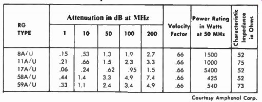
Table 6-1. Attenuation per 100 Feet of Common Coaxial Cables
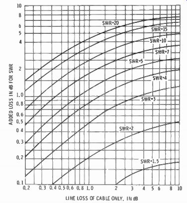
Fig. 6-6. Chart shows additional loss in dB when the SWR is greater than 1:1.
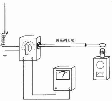
Fig. 6-7. Recommended instrument hookup when adjusting the base loading coil
on a vertical antenna.
Table 6-1 listing popular feeders shows the attenuation in dB for each 100 feet of cable at various frequencies. From this you can see that long cables at very-high frequencies can mean a considerable loss of power; this is power that dissipates as heat in the line and never gets to the antenna. In addition a high SWR can increase the losses because of the higher voltages resulting from the higher SWR. The chart in Fig. 6-6 shows the added dB loss resulting from SWR ratios higher than 1:1. This figure is added to the dB figure based on length and frequency for a figure of total loss. For example: A 50-ft. length of RG-58/U cable has about a 2.3-dB loss per hundred feet at 30 MHz. The center of the antenna was measured to have an impedance of 73 ohms at resonance (a perfect situation). The nominal characteristic impedance of the cable is 53.5 ohms. The 73 SWR because of mismatch is or 1.36:1 by calculation. From the chart of Fig. 6-7, it can be seen that the additional loss because of this mismatch is so small as to be off the chart, therefore insignificant. The loss due to line length is one-half of 2.3 dB (for 50 ft) or 1.65 dB. Converted to power loss, as obtained from any power versus-dB chart or table or using a slide rule or logarithmic table, mathematically, we solve for:
dB = 10 log
where, Po is power into the feeder, P] is power into the antenna.
Therefore, one-tenth 1.65 is .165, and the antilog of .165 is 1.46. This means that for every watt into the antenna, it takes 1.46 watts into the feed line based on cable type, length, and frequency only. however. if the SWR is 3:1, the chart will show that an additional 0.6 dB of loss must be added to the 1.65-dB figure, for a total loss of 2.25 dB. The log tables will show it takes 1.67 watts into the feeder to get 1 watt into the antenna, or about 40 percent of the power is lost in the cable compared to a 31.5-percent loss from the cable alone. The RG-58/U is obviously not a good cable for long lines at high frequency. A better choice would be the popular RG-8/U.
TUNED LINES
All that has been said about antenna resonance and its measurement with a half-wave line applies only to "matched" type or untuned lines, whether balanced (parallel-wire type) or unbalanced (coaxial type). The output of most transmitters is designed for direct unbalanced connection of a 50-ohm line, which is the most popular line in use. However, tuned feeders are still popular with many amateurs and have the advantage of multiband operation without the use of antenna traps, and the use of tuned feeders reduces the problems of resonating the antenna precisely. The disadvantage of tuned feeders is the need for careful installation, particularly with regard to the method by which they are brought into the shack from the outside. Also, tuned-feeder systems require an antenna tuner in the shack, which is used to resonate the system and couple it to the transmitter. When a tuned feeder is connected to the center of a dipole, there is no need to trim the antenna to exactly one-half wave length. It is sufficient to cut approximately based on the standard formula for antenna length. With the feeders connected to the center, currents and voltages in the two legs of the feeder will always cancel and radiation is only from the antenna. Of course, standing waves will be high on the feeder, but wide-spaced conductors with good insulating spacers keep losses down. Even if the antenna length is off, there is always balance in the line. And since the entire system (antenna and feeder) is resonated at the antenna tuner, resonance for any frequency is easily accomplished.
"Zep"-fed (end-fed) antennas can result in some unbalance in the feeder if the antenna is not at resonant length. While an end-fed antenna with tuned feeders can be still be resonated with the antenna coupler system in the shack, if the antenna length is too far off there will be unbalanced voltages and currents in the feed line and some feed-line radiation. Usually that unbalance is not important enough to go through a lot of trouble to achieve exact resonance of the antenna, and the formula for cutting the antenna mechanically is good enough.
TUNING A VERTICAL
A vertical antenna is considered to be a quarter-wave antenna with the ground acting as the other quarter wave when the antenna is fed at the point where the vertical connects to the ground, usually right at the ground point. Because of the conductivity of the earth where radials are buried in it, and the infinite length of cold-water pipes when they are used as the ground, the total length of the antenna is anything but a halfwave, or twice the vertical quarter-wave.
You might say it is resonant at any frequency, and tuning means shifting the center current loop to the feed point at the frequency you want to operate.
The length of a simple vertical is based on the formula: 934 L (ft) = f (MHz)
Vertical antennas can be tuned to precise frequency (current loop at the feed point) with a small reactance (either capacitive or inductive) in series; a variable capacitor in series if the antenna is too long, or an adjustable inductance in series if it is too short. Because of their height, vertical antennas can become pretty clumsy in the lower amateur bands. They are common for mobile operation on 10 meters, but for fixed or mobile operation at lower frequencies, short verticals with base-loading coils or traps are more common. For very short dimensions (as for mobile operation) better performance is obtained if the loading coils are up higher in the antenna. Since the area of maximum r-f current in the antenna is the most effective radiator, it should be left free to become part of the vertical antenna portion.
Common low-frequency verticals for fixed-station operation have resonant traps which give them multiband resonances as well as shortening the overall length. These are not subject to tuning when purchased complete.
Among home-made fixed-station verticals the most common is the short vertical rod (usually about 22 feet high and base-loaded with a tapped coil). Trimming the antenna means adjusting the tap on the coil for the purpose of placing the current loop at the feed point.
While a perfect vertical without lumped inductances and with a perfect ground of a number of buried radials typically has a center impedance of about 30 ohms, the shortened version with a base-loading coil, especially if the ground system is not perfect, can have a center impedance as high as 200 ohms. With a poor ground it is sometimes impossible to find resonance by coupling a GDO to the antenna at the feed point. The best method is to use the GDO as a signal source and adjust the antenna for the lowest impedance at the feed point with an impedance bridge. Fig. 6-7 is the hookup for tuning a one-band vertical with a base-loading coil. This hookup is for rough adjustment at the antenna. The feed line must be a half wavelength long at the operating frequency in order to show the same impedance at each end.
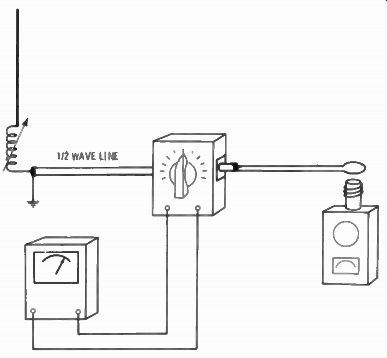
Fig. 6-8. After adjusting the vertical with the setup of Fig. 6-7. bring the
impedance bridge into the shack for the final touchup.
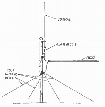
Fig. 6-9. When good grounding is impractical, quarter wave radials above ground
will give superior results.
Set the GDO to the operating frequency at the shack end of the line.
Adjust to nearly exact frequency by listening to the beat in the receiver with the bfo on. Connect the impedance bridge and meter between the feeder and the feed point of the antenna. Adjust the taps on the coil, at the same time varying the bridge arm for lowest reading on the balance meter. Disconnect the bridge and reconnect the feed line. Bring the bridge inside and connect it as shown in Fig. 6-9.
This time juggle the bridge arm and the frequency setting of the GDO for lowest reading on the bridge meter. You will probably find that a complete zero can be obtained at a frequency slightly off the frequency at which you first set the GDO for the outdoor check on impedance. If the frequency of perfect bridge balance is higher than the desired operating frequency, add a little inductance to the base coil at the antenna. If lower, move the tap to reduce the inductance.
You may find that even only a quarter turn on the coil will make a big shift in frequency. Your antenna is resonant to the desired frequency when the meter balance is zero, and the antenna impedance is the impedance read from the bridge arm. That impedance may be anything from about 30 ohms to 200 ohms; but regardless of the impedance, the antenna is resonant, which is the important thing. If the impedance happens to come close to the characteristic impedance of the feed line, the mismatch is unimportant and can be ignored.
If the mismatch is 2:1 or greater, check for power loss as described before in this section, and correct the mismatch if power loss is excessive. The power loss will depend on the operating frequency, the quality of the feed line, and its length When the impedance bridge is connected to the base of the vertical as shown in Fig. 6-7 it introduces discontinuity and stray capacitance or inductance that may prevent obtaining a zero balance on the impedance meter. With the bridge at the input end of the cable, the normal operating connection at the antenna gives better balancing results (Fig. 6-8). If the resulting impedance is far from the 30-ohm average of a vertical antenna, it is because of the use of the lumped inductance at the base of the antenna, a less than perfect ground, or the use of an unbalanced cable (coaxial cable, for example) connected to a probably balanced feed point. Although the antenna is resonant (and this is most important), the mismatch to the cable characteristic impedance may result in a greater-than-desired power loss, and an in ability of the transmitter to load properly.
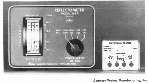
Fig. 6-10. This reflectometer has a meter with two pointers. One reads forward
power and the other reflected. When loaded with exactly 50 ohms, the power
readings are actual. VSWR is shown in the vertical panel scale to the right
of the meter. Courtesy Waters Manufacturing, Inc.
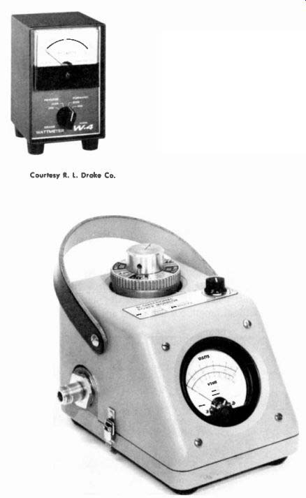
Fig. 6-11. The Model W-4 Wattmeter reads actual power into a 50-ohm load. Flipping
a switch changes the reading from forward to reverse power. A calculator, supplied
with the instrument is used to convert to SWR.
Fig. 6-12. The Sierra Bidirectional Power Monitor reads forward power and SWR directly on the meter scale. Plug-in units, on top, are multipliers for reading power in watts into a 50-ohm load. Courtesy Phiko-Ford Corp
ABOUT VERTICAL ANTENNA GROUND
Probably the most important consideration in the performance of a vertical antenna is a good ground. In many areas of the country, such as the Southwest where the climate is dry and the soil sandy, buried radials of random length for a ground are almost useless. Unless the buried radials are themselves a quarter-wave long it is better to use above-ground radials (Fig. 6-9). With the antenna up in the air, and about four quarter-wave radials coming off at about 45°, you will have less trouble finding resonance and matching the impedance. The center impedance of an antenna built like this is about 72 ohms.
THE SWR METER
The antenna impedance bridge described previously cannot be left in the feed line while operating the transmitter. A device for indicating relative output power and SWR that can be left in the line is the SWR meter (Figs. 6-10, 6-11, and 6-12). The construction of one is described and shown in the next section. The circuit diagram is duplicated in Fig. 6-13 for illustrative purposes. The SWR meter reads Fig. 6-13. Circuit diagram of the SWR meter described in Section 7.
the forward-going wave and the reflected wave which is due to mis match, and from this information the SWR ratio is obtained. The values of R, and R. arc selected for use on a particular line characteristic impedance, and the readings will be true only when the line used between the SW R bridge and antenna has that impedance.
The SWR or standing-wave ratio is a function of the forward voltage versus the reflected voltage, and it is based on the following formula:
SWR = Vo + Vr, v 0 - VR where, V o is the outgoing voltage, V R is the voltage value of the reflected wave.
The voltage need not be absolute, but only relative. For example, the forward voltage is at full scale of the meter, which is 1 on a 100-
/*A meter.
Switching to reflected wave the needle reads 0.5, or mid scale. Substituting in the formula:
SWR =
= I 5 .5
= 3
A handy device for reading SWR directly is the chart of Fig. 6-14.
USING THE SWEEP GENERATOR FOR ANTENNA RESONANCE
An excellent method for "seeing" the results of antenna off-resonance and adjusting for resonance is through the use of a sweep generator and scope, employed in the same way as using a sweep generator for aligning a receiver. In this case it is the resonance of the antenna that is under investigation.
The sweep generator connects to the same bridge as used previously. It is the signal source, but it sweeps a range of frequencies instead of supplying a single frequency. The balance indicator is a scope instead of a meter. The horizontal sweep of the scope is synchronized with the sweep of the generator. As the generator sweeps past the point of antenna resonance the scope will show a dip in the trace, which is equivalent to the zeroing of an indicating meter. The trace will look something like Fig. 6-15 À or B. In Fig. 6-15A the dip is easily recognized. In Fig. 6-15B the dip is inverted and looks like a peak, but it is a dip nevertheless. It is inverted because of the number of stages in the scope and is a matter of phase. Consider the trace with relation to the base line, regardless of the direction. Fig. 6-16 is the hookup for using the sweep. It is similar to the hookup using a straight signal generator and a microammeter balance indicator, except for the type of instruments. If the sweep generator does not have a built-in marker oscillator, it will be necessary to use one externally. The marker generator places a pip on the trace and is the method for determining exact resonance of the antenna. Many sweep generators have facilities for plugging in a crystal for marker purposes. An amateur-frequency crystal for the band for which you are trimming your antenna is an excellent marker.
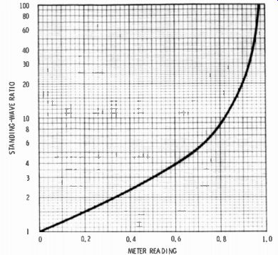
Fig. 6-14. A chart like this can be used with any meter scale. Adjust the
forward reading to 100-percent of scale, and convert reflected reading to SWR
from this chart. Courtesy Allied Radio Corp
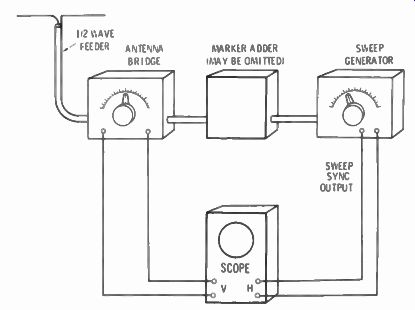
Fig. 6-16. Hookup for using a sweep generator and scope to observe antenna
resonance.
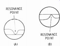
Fig. 6-15. Appearance of the dip on a scope indicating antenna resonance with
a sweep generator. The customary dip is at A. At B it appears as a peak, but
it is the "dip." The difference is the result of phasing.
For this method the sweep generator must have fairly high output, and the scope must have good sensitivity but not necessarily high frequency response. There is considerable loss of signal in the bridge and it takes about 1-volt output from the generator, plus a sensitivity of about .025 V/inch on the part of the scope, to get a normal-sized pattern. No demodulator probe is necessary for the scope since the rectifier in the bridge acts as one.
Set up the sweep generator for about 2-MHz sweep width, and the place the tuning dial to the frequency at which the antenna is to be measured. Place the bridge control arm at about 50 ohms. The pat tern you will see will be nearly like one of those illustrated here, but the dip will probably not touch the base line. Now adjust the balance arm on the bridge until the dip touches the base line. The reading on the bridge arm will be the impedance of the antenna at the center, and the point where the dip touches the base line is the resonant frequency. Turn up the gain on the crystal marker (if one is used ) and see where the pip appears. If an external variable signal generator is used as a marker, adjust it until the pip appears at the center of the dip. The frequency of the marker generator is now at, or near, the resonant frequency of the antenna.
If resonance appears at a frequency other than the frequency for which the half-wave feed line was cut. reactance in the feed line will affect the exact resonant frequency. However, an antenna resonance off the desired frequency of operation is indicated. How far off and the direction is the real point of interest. When the antenna is trim med to the desired operating resonance (equal to the half-wave length of the feeder), the frequency will be correct.
Fig. 6-15B was drawn from an actual test for resonance of a new 40-meter vertical antenna. The off-center marker pip was from a 7.150-MHz crystal. It indicated that antenna resonance was too low, and needed trimming to bring the peak of the dip (inverted here) at the pip marker.
A variable marker can be moved back and forth on the scope screen to determine how broad the antenna resonance is. If you experience intermittent waviness in the trace lines, it is the result of a close-by broadcast station.
FRONT-TO-BACK ANTENNA RATIO
Beam element length and spacing, as given by standard formulas or supplied by the manufacturer (if purchased) usually provide results so nearly optimum it does not pay to make field adjustments.
However, it is sometimes desirable to know that everything is working as it should. Resonance and feed-point matching measurements are made as described before. Forward-gain measurements or front to-back measurements require some means of picking up the forward and rear power and comparing them. This is done with a field strength meter whose pickup antenna is placed in front of the beam at least three wavelengths away.
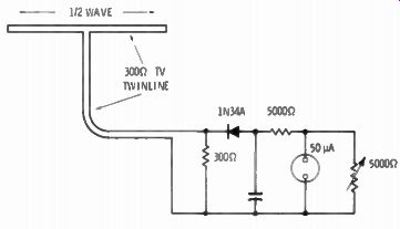
Fig. 6-17. Field-strength meter using 300-ohm TV twin-line as a dipole and
feeder.
Fig. 6-17 is the sketch of a simple field-strength meter for this purpose. It consists of inexpensive 300-ohm TV twin-line, both as a dipole and a feeder. At the end of the feed line is a 300-ohm load resistor, followed by a rectifier, r-f bypasses, and a sensitive meter. A variable shunt across the meter reduces sensitivity for higher-power transmitters. A series resistor is needed for obtaining linearity in the meter reading because of the nonlinear characteristics of the diode.
It reduces sensitivity, of course, and may be eliminated if only a relative reading rather than an absolute reading is acceptable. The meter may be a 50-/zA to a 1-mA type depending on need for greater sensitivity. If a 50-juA meter is used, the variable shunt resistor should be 5000 ohms, down to 200 ohms for a 1 -mA movement.
Where high sensitivity is not necessary the pickup antenna need not be a full half wave. The entire r-f portion may be built on a plastic board with short dipole elements sticking out each end, all the r-f components on the board, and any kind of lamp cord feeding away to the meter located nearer the antenna so it can be seen if adjustments are made. The meter may be mounted to the board also if any F/B (front-to-back) measurements are to be made.
The field-strength dipole must be hung parallel to the antenna under measurement. It is important that polarization be the same.
Unless the field-strength dipole is hung several wavelengths away from the transmitter antenna it may be part of the inductive field and affect the antenna dimensions. The field-strength antenna feeder must be brought away from its dipole at right angles; it must not pick up signal from the transmitter. The same is true of the transmitting-antenna feeders; they must not radiate energy. If the antenna is not gamma-matched or does not use a balun (if feeding a balanced antenna with unbalanced coax), the feeder is apt to radiate and give wrong readings.
If the series resistor is used on the meter, the meter readings may be taken as a measure of relative voltage. Rotate the beam to point to the field-strength antenna, and adjust the meter for full-scale reading (E,). If it cannot be adjusted to full scale, note the reading.
Rotate the beam to point in the opposite direction and note the meter reading (E.). Convert the readings to dB with the following formula:
p dB = 20 log E 2
where,
E' is field-strength reading off the front,
E- is field-strength reading off the back.
If you make adjustments to the elements of the beam, remember a few things: Increasing the recommended length of the reflector often results in increased F B ratio, but not an improvement in power gain.
Best F/B ratio is seldom the same as best power gain. Any adjustment to any element will affect the length of other elements. Recheck particularly the driven element for resonance and feed-point match.
If the driven element needs adjustment, go back over the other elements again. You may find it necessary to repeat the adjustments to each element until a nearly perfect ratio (resonance and feeder match) is obtained.
MATCHING TRANSMISSION LINE TO ANTENNA
A feed line of the untuned type has a characteristic impedance based on physical dimensions determined by the diameter of the conductors and the distance between them. When terminated by a pure resistance equal to the characteristic impedance, there are no standing waves and loss is at a minimum. The center of a resonant antenna is a pure resistance, and when its value is the same as the characteristic impedance of the feed line, a direct connection can be made.
When the antenna impedance is different from the line impedance, standing waves will be set up in the line, and the losses will go up. If the mismatch is great enough, the losses become important enough to do something about correcting the mismatch. There are three popular methods of correcting the mismatch.
THE GAMMA MATCH
One of the most convenient and effective (and most popular) methods of matching the low impedance of the driven element of a beam is the gamma-match method. In addition to increasing the feed point impedance, it provides for changing from a balanced antenna center to an unbalanced coaxial cable. The diagram is shown in Fig. 6-18.
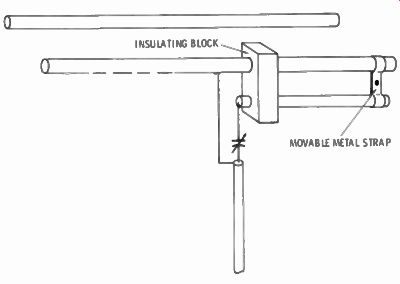
Fig. 6-18. One of the most popular methods of matching a coaxial cable to
the center of the driven element of a beam is the gamma match. Adjust the position
of the slider and the value of the capacitor for a 1:1 SWR. Voltage is low
at the feed point, so the capacitor may be a receiving-type variable.
The half-wave driven element is not broken in the center, but is made continuous. A similar aluminum rod is supported about two inches below the driven element, extending from the center to about 40 percent of the length of one side. It is insulated from the driven element at the center. At the far end is a metal support, which is constructed to permit sliding it up and down the matching element.
The shield side of the coaxial-cable transmission line connects to the center of the driven element. The inner conductor connects to a variable capacitor (about 150 pF for 14 MHz; more for lower frequencies, less for higher frequencies) connects between the inner conductor and the beginning of the matching element. Since the matching element is shorter than a quarter wave, it will have inductive reactance. The capacitor tunes this out.
Adjustment is made by sliding the end strap back and forth, and at the same time adjusting the variable capacitor, until an SWR of 1:1 is read at the input of the transmission line.
THE Q-BAR
A quarter-wave length of feeder open at both ends acts like a transformer. When it is terminated in its characteristic impedance at one end, the other end will look like the same impedance. When the one end is terminated in an impedance higher than its characteristic impedance, the other end will look like an impedance lower than its characteristic impedance-thus the transformer action. For matching feed lines to antennas, this quarter-wave section has been popularly known as a "Q-Bar."
Two unequal impedances can be matched when the impedance of the Q-bar has a characteristic impedance that is the mean value between the two unequal impedances. The formula is: 2q = 21 X 2 2
For example, the center of a resonant antenna was found to have an impedance of 200 ohms by measurement with an impedance bridge as previously described. It is desired to match a 50-ohm line to that antenna. Using the above formula the Q-bar impedance must be:
Z^ = \/ 200 X 50
= V 10,000
= 100
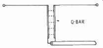
Fig. 6-19. The usual (9-bar quarter wave matching section consists of parallel
conductors, spaced with insulators. The desired impedance of the ß bar can
be predetermined by formula, and constructed by spacing and radius of the conductors.
A O-bar is usually made up of a pair of parallel conductors one quarter wave long (Fig. 6-19), and its characteristic impedance is reached by observing the following formula:
d = 276 log - where,
d is the distance between conductors, center-to-center, r is the radius of the conductors.
Once the O-bar is made to the above dimensions the exact quarter wave length can be measured by shorting one end and coupling a GDO to the short. Start with a length slightly longer than a quarter wave, and cut from the open end while checking the frequency of the dip on the GDO until resonance at the operating frequency is reached.
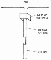
Fig. 6-20. Under certain conditions, coaxial cable may serve as the quarter-wave
matching transformer.
Although parallel bars can be constructed to meet a specific imped ance need, it is sometimes possible to find manufactured cable to meet the impedance needed for a quarter-wave Q-bar. Fig. 6-20 shows one example. The center of the driven element of a beam was found to have an impedance of about 37 ohms. By using an electrical quarter-wave length of 52-ohm coaxial cable, an impedance trans formation was made to 73-ohm coaxial cable for the feed line.
MATCHING STUBS
When the transmission line and antenna feed point are mismatched, there will be standing waves along the line. By attaching a prescribed length of feeder at a prescribed distance down the feed line, the reactance of the unmatched line can be "tuned-out," and at the same time a value of impedance created at the junction that will match the line. This is known as stub-matching and it looks like Fig. 6-21 for both open lines and coaxial cable.
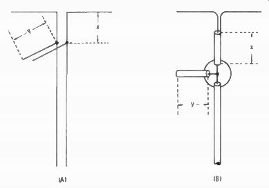
Fig. 6-21. Matching stubs may be added to open transmission lines (A), or
to coaxial lines (B). Dimensions for X and Y are obtained from formulas and
the SWR before correction.
The length of the stub and the point of attachment is determined by formulas. The only thing we need to measure beforehand is the SWR between the unmatched line and antenna as determined by the ratio indicated on an SWR meter.
Connect the feeder directly to the center of the antenna in the usual way. Measure the SWR at the input of the line (at the transmitter). (Note: when using coaxial cable, which is an unbalanced transmission line, better results will be obtained if a balun is added to the balanced center of the antenna. A balun changes the balanced center to an unbalanced line, and prevents rf from appearing on the outside of the line. The most convenient is a balun transformer wound on a toroidal ferrite core. These may be purchased or you can make your own from information in amateur radio handbooks.) The following formulas are for use where the stub is made of the same type line (that is, same impedance) as the transmission line.
Working out the formulas will give the distance (X) and length of stub (Y) as shown in Fig. 6-22. First, solve for length in degrees, then convert degrees to electrical length at the desired frequency.
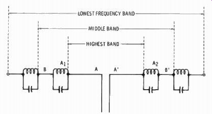
Fig. 6-22. All-band trap antennas use tuned circuits to isolate the higher
band from the next lower band. At a lower frequency, the inductance of the
higher-band traps become part of the added elements.
Where the antenna impedance is greater than the line impedance, the formula is:
tan X - SWR and SWR - 1 cot Y = \/SWR
Where the antenna impedance is less than the line impedance, the formula is:
cot y = s/SWR and tan Y = SWR - 1 V SWR
The degrees obtained from these formulas must be converted to electrical length from:
degrees = 360 times length in wavelengths
The answer will be a decimal fraction of a wavelength, which is added to the standard formula for length in feet:
Length in feet 984 X V , . X wavelength decimal f (MHz)
where, V is the velocity factor of the cable,
f is the frequency.
Example: A 52-ohm coaxial cable is to feed the center of the driven element of a beam. The SWR reading before any correction was applied is 3:1. The coaxial cable has a velocity factor of .66, and the frequency of operation is 14.25 MHz.
tan X = v/SWR = V3 = 1.7321
Checking a trigonometry table, or using the slide rule, the angle for which tan X = 1.7321 is 30°. 30° is .083 times 360°. The length in feet of section X, or the tap on the line will be: 984 V X (feet) = r X .083 / (MHz)
* - = 3.81 feet
Therefore, distance X will be 3 feet 9% inches from the antenna feed points, for operating at 14.25 MHz.
The stub length ( Y) for the same case is: SWR - 1 cot Y - \/SWR 3 - 1 2 1.7321 = 1.155.
The angle for which cot Y is 1.155 is 41° (approx). The angle 41° is .114 times 360°. The length in feet of stub Y will be: 984 V , 984 x 66 X ,H4 14.25
= 5.18 feet, or 5 feet 2+ inches
Because the stub Y is shorter than a quarter wave, its reactance tuned out the reactive component of section X, so that the line is looking at a pure resistive load of 52 ohms at the junction. While standing waves will appear on the length X plus Y, the feed line will be flat and should then show a 1:1 SWR ratio at the transmitter end.
ANTENNA TRAPS
A popular method of constructing a multiband antenna is with resonant traps. Fig. 6-22 shows a dipole for three-band operation using two pairs of traps. Traps also reduce the overall length.
The dimensions of sections A and A' of the sketch are tuned to the frequency of the highest band as if there were no traps or other element lengths there. Traps A) and A 2 are parallel-resonant tuned circuits. Their resonant frequency is the frequency of the highest band, or dipole section A-A'. The high impedance of the parallel resonant trap isolates the high-band dipole (A-A') from the rest of the elements when a signal of that frequency is fed to the antenna.
For the next band, the traps are no longer resonant but do represent an inductance in series with the elements of A and A'. Elements B and B' are added and tuned to the next or middle band. The middle band dipole now consists of B-A1-A2 and A'-A2 -B' resonant to the middle band. Another pair of resonant traps tuned to the mid-frequency of the second band are added, followed by elements to resonate to the lowest band with all the elements of the high band, middle band, and the inductances. Thus we have a three-band antenna, resonant to each of three band frequencies fed to it from the same feed line and the same center feed point.
Traps can be set precisely to frequency by coupling a GDO to the coil and adjusting to resonance, provided the coils are not enclosed in a metal sleeving, as some are. You can make your own traps from air-wound coils and parallel capacitors, setting them to frequency with a GDO. Enclose the combination in a polystyrene sleeve for weather protection. All this can be done in the workshop ahead of time. Except for the highest-band elements, which may be cut to the standard formula, the rest is cut and try. The elements added beyond the highest band elements must be determined experimentally be cause the inductance added by the nonresonant traps depends on the ratio of L to C; the higher the L is, the shorter will be the added elements.