There is hardly a QSO on the air that does not include a report on the transmitter being used, and power rating of that transmitter. Power is the standard of comparison between transmitters. A power of 1 kW is the legal limit of input for amateurs in the United States.
Power is work, it is energy, and when used right, it is what pushes effective radio waves off the antenna. Power is the result of voltage (E) forcing current (/) through a load (R). It is expressed in various ways by Ohm's law:
P = IE
P = I^2 R
P = E^2 / R
These expressions will be used in considering power measurements.
DEFINITIONS OF POWER
The most common understanding of power by amateurs is the input power to a continuous-wave generator which is the output stage of a transmitter. With key down on a c-w rig, or unmodulated carrier on for an a-m phone rig. the input power is simply the plate voltage times the plate current (P = EI).When an a-m rig is modulated, power is being added to the carrier in the form of sidebands. Each sideband, for 100-percent modulation, is equal in power to 25-percent of the carrier. Thus, for 100-percent modulation, a modulator must have a power capability equal to 50-percent of the r-f output-stage power capability. A kilowatt rig is putting out the equivalent input of a 1500-watt rig. when it is 100-percent modulated. The 1-kW limit is exceeded technically but not legally. Rated input power is still E times / to the r-f amplifier, whether modulated or not.
Measurement, therefore, is simple-multiply the plate current reading by the plate voltage on c-w and a-m phone transmitters. Do not hold the key down too long on a c-w rig, or you may be damaging the final tube. A c-w transmitter is designed for intermittent service if it is designed to give the most for the money, and closing the key could cause the final tube to overheat. In a well-designed a-m phone rig, the power-input reading should not be affected by whether the rig is modulated or not--the plate current should be the same.
The input power to an ssb transmitter is a little different. There is no carrier until the transmitter is modulated. But FCC regulations for setting the legal 1-kW limit are liberal. They will accept the reading of plate current and voltage during modulation, provided the current meter does not have a time constant longer than 0.25 second. Under these conditions it is still plate voltage times plate current on the final. So if you are running a 1-kW ssb transmitter, use a plate current meter with a 0.25-second time constant and keep your eye on it while modulating. Most commercial milliammeters have about the right time constant.
AC POWER OUT
Up to now we have been talking about the power supplied to the final by the power supply; it has been all DC power. But DC power does not indicate the amount of power coming out of the final stage into the antenna for a signal. R-f power can be measured with an r-f ammeter or an r-f voltmeter, and can be "seen" with an oscilloscope. R-f power output will be something less than the DC power input-no r-f amplifier is 100-percent efficient. As a starter let's "look" at the rf with a scope, and see what goes on.
CONNECTING AN OSCILLOSCOPE
The frequency of the r-f output of a ham rig is much too high for the input amplifier of the average scope. Many moderately priced scopes have a vertical-amplifier response that is flat up to around 5 MHz, and these could be used at 80 meters. But to see r-f at higher frequencies, you must apply the r-f directly to the vertical-deflection plates of the cathode-ray tube. Many scopes have direct access on the back of the case where the terminals of the deflection plates are brought out to jumper bars. By removing the jumper bar of the vertical plates, direct connection can be made. If this feature is not on your scope, install a connection just for the vertical-deflection plates.
Remove the scope from the case. Solder a 0.01-uF disc capacitor to each of the two socket terminals of the CRT vertical-deflection plates. Cut a hole in the back of the case (if there is not already an opening), and bring the two capacitor leads out to a two-terminal tic point, or to binding posts. This type of connection does not interfere with the normal centering controls on the scope, and it leaves the scope free to be used for other oscilloscope duties. Fig. 5-1 ...
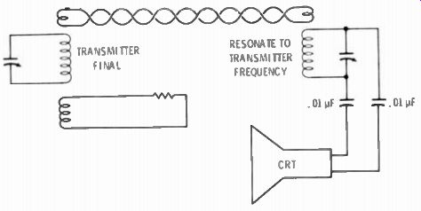
Fig. 5-1. The most effective way of coupling a transmitter to the vertical
deflection plates of an oscilloscope.
... shows the r-f pickup circuit. A two-turn loop permits you to adjust the voltage by varying the coupling to the final tank coil, but observe caution in handling, since you arc in the presence of high voltage.
The resonant circuit tunes to the signal frequency for maximum signal to the scope. Often there will be enough r-f pickup by connecting to the center lead of your output coaxial cable. Use a Tee coaxial connector for this. It may be possible to eliminate the tuned circuit, depending on the power of the transmitter and the deflection sensitivity of the CRT in the scope. Simple capacitive coupling may be enough.
The transmitter must be fully loaded with a dummy load. Don t clutter up the air with unnecessary signals while you are making transmitter observations or measurements, except when it is required that the antenna be connected. Adjust the pattern size by the loop coupler and/or the tuning of the resonant circuit. Fill about 2/3 of the CRT with vertical deflection with the internal sweep on the scope set at a slow rate of about 30 Hz.
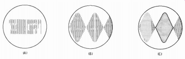
Fig. 5-2. Pattern on scope of a c-w signal is shown at A. This is also the
pat tern obtained by modulating an ssb rig by a single audio tone. B is the
pattern of an a-m transmitter modulated by a 1000-Hz tone, and an ssb transmitter
with a combination of two tones 1000 Hz apart. C outlines the power portion
of an ssb signal.
WHAT YOU SEE
The trace for a c-w signal will look like a bar (A in Fig. 5-2). The height from top to bottom is the peak-to-peak relative value of the r-f voltage. The rms value, if the signal is a pure sine wave, is the peak-to-peak voltage value divided by 2.828. At the moment the actual value has no meaning. Modulate an a-m rig with a pure 1000-Hz tone from an audio generator, and the pattern will look like B in Fig. 5-2 at 100-percent modulation. The total height of the pattern doubles. At double the voltage, the instantaneous peak power is four times the unmodulated power, since power varies as the square of the voltage (P = E^2 /R). It is the doubling of the voltage during modulation that accounts for the need for high-voltage r-f output capacitors in phone rigs as compared to straight cw. Modulate an ssb transmitter with a single 1000-Hz tone and it will look like a c-w carrier (Fig. 5-2A). What is observed in Fig. 5-2A is the side band only, or an r-f signal whose frequency is the basic suppressed carrier plus 1000 Hz. For example, 3.9 MHz plus 1000 Hz equals 3.901 MHz, and that is what you will see. But, modulate an ssb transmitter with two tones simultaneously, and it will look like B of Fig. 5-2. Here you are seeing the effect of two r-f signals and the beat between the two. In our example a 3-kHz tone and a 4-kHz tone beat with 3.9 MHz will produce signals of 3.903 MHz and 3.904 MHz, and the beat between 3.903 and 3.904 MHz is 1 kHz. The two-tone test is the most popular test for adjusting an ssb transmitter for proper linearity. The ssb pattern shown helps to explain what is meant by PEP for an ssb transmitter. PEP means peak envelope power, and is the power shown under one curve on the pattern out lined in bold in Fig. 5-2C. It is not the instantaneous peak mentioned before, but the power at modulation peaks. At the time it occurs it is about twice the equivalent DC input-power average. This accounts for the 2000-watt PEP ratings of ssb rigs in the 1-kW class.
POWER EFFICIENCY
Outside of the need to know that the legal limit of 1-kW DC input to the final is not being exceeded, the real concern with power is to know how well the transmitter is doing in getting a signal into the antenna and out on the air.
The efficiency of the output stage is a ratio of the r-f power output to the DC power input to the last stage. It may be expressed as:
Eff = = P_out_/Pin
A class-C amplifier runs about 75-pcrcent efficiency. A class-B amplifier as used in ssb transmitters runs about 65-percent efficient.
These are typical maximums. The difference between power in and power out is heat, heat that must be dissipated by the final tube or tubes. It is the ability to dissipate this lost heat that determines the rating of the tubes used as final amplifiers. Coupling to the output also enters into efficiency, and optimum coupling is obtained when the load impedance of the tube is matched.
The maximum power which can be fed into a tube or set of tubes is the highest voltage the tube will take without arcing over, times the current at saturation, above which there just can be no increase in the electron flow from the cathode or filament. Operating a tube under saturation conditions will result in calling on the tube to dissipate much more heat than it is designed for. But another factor enters the picture, and that is time on. If the tube has a short on-time cycle it can handle more heat dissipation for that moment than if it is required to throw off the heat continuously. With this in mind tubes may be operated above their continuous-duty ratings when keyed for cw, and when used in ssb transmitters. In a-m phone the carrier is on all the time the transmitter is in transmit mode, so the final tubes must be used within their normal rating if a long life is expected.
MEASURING POWER OUT
Output power may be measured by an r-f ammeter, or r-f volt meter. Most r-f ammeters read the voltage developed in a thermo couple through which the rf is flowing. An r-f voltmeter is a VTVM
with an r-f probe, designed to read the r-f voltage in a rectifier circuit in terms of the DC it develops. Some VTVM's have a vacuum tube diode in a special probe; others use a solid-state diode in the probe. You can build your own probe from the circuit shown in Fig. 5-3. The components must be shielded from stray pickup. An excellent enclosure is the tube shield of a miniature tube. After the components are wired in a tight bundle and a shielded cable is connected to the output, place the circuit into a tube shield with a test probe sticking out the top and pour an epoxy filler into the tube shield. The epoxy is available at many of the leading radio- and TV-parts supply companies. The VTVM is set on its DC function. The DC reading on the scale will be approximately correct for the rms value of the rf.
SHIELDED CABLE TO VTVM
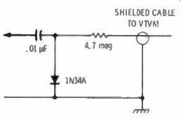
Fig. 5-3. Circuit of an r-f or demodulator probe. With these constants a VTVM
will read the peak value of rf on the DC scale.
Diodes in r-f voltmeters are limited as to the voltage they can handle, and this limit must be observed. On solid-state diodes the limit on most is about 20 volts. A resistor voltage divider must be used externally for reading higher voltages. VTVM's with vacuum tube diodes are usually good for reading voltages up to about 500 volts without damage to the diode. In the voltage divider circuit of Fig. 5-4, the voltage out is related to the voltage in by the value of R2 to the sum of R1 and R2 . This ratio can be simplified as follows:
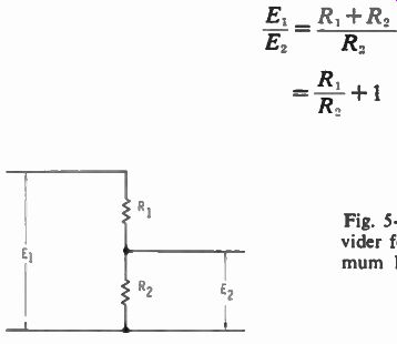
Fig. 5-4. A carbon-resistor voltage divider for reducing rf to the low maximum limits necessary for instrument demodulators.
... or: E2/E1- 1 = R1 /R2
Thus if the ratio of E1 to E2 is to be 10 to 1, subtract 1 from the ratio, which makes it 9 to 1 as the ratio of R1 to R2. For example a voltage divider using 6200 ohms for R, and 670 ohms for R2 will provide about a 9-to-1 resistance ratio, or a 10-to-1 voltage division. These values must be selected from 5-percent carbon resistors. This example is a good one for use on 52-ohm coaxial lines, for output wattages to 800 watts. To maintain accuracy and prevent phase shift, keep the leads short and the input and output well separated from each other.
A handy replacement for an r-f ammeter is a resistor in series with the output, across which the voltage drop is measured and then converted to current by I = E/R. Having the current, calculate power by P = I^2 R.
A 1-ohm, 2-watt carbon resistor in series with the ground side of the r-f output (the ground side because the metal case of the VTVM could be accidentally grounded) deducts very little from the output and gives you the equivalent of the circuit shown in Fig. 5-3. The r-f probe converts the high-frequency rf to de, which is then read on a low DC scale of the VTVM. A 2-watt resistor will handle up to 2 amperes of current. Into a 50-ohm coaxial load, powers up to 200 watts may be read (P = PR = 2- X 50 = 200). For higher power, a higher-power resistor must be used. Four 1-ohm 2-watt resistors in series-parallel will handle 4 amperes, or 800 watts output.
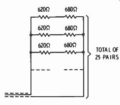
Fig. 5-5. A 52-ohm, 100-watt dummy load can be made up of paralleled 2 watt
carbon resistors.
THE DUMMY LOAD
According to Ohm's law you will need another value in addition to current or volts, and that is resistance (R). The resistance is the output load impedance when the antenna is at resonance and the feeder is perfectly matched to the antenna, or a dummy load that is nonreactive and of known value. If these conditions are not met the load impedance will be more or less reactive and the reading will not give you true power output. It is obvious from this that initial measurements and adjustments should be made into a nonreactive dummy load. A dummy load can be made up of a combination of carbon resistors in parallel or series-parallel. Power handling will depend on the number and rating of the resistors. Fig. 5-5 shows the assembly of 2-watt carbon resistors to make a 100-watt dummy load. Purchase twenty-five 680-ohm 10-percent resistors and twenty-five 620-ohm 5-percent resistors (620-ohm resistors come only in 5-percent types), and connect a 680- and a 620-ohm resistor in series. Connect the 25 series-connected pairs in parallel. Keep pigtails short and stray capacity low. Connect a coaxial cable to the ends as close as possible. From about 14 MHz up, this dummy load will begin to show some reactance, because the total length of the bundle will act like a wire loop. For amateur use at the usual lower-frequency bands this makes a fairly nonreactive dummy load, and the net load resistance will be 52 ohms. Higher-powered dummy loads are constructed similarly, but with higher wattage resistors or more of them. Dummy loads are available commercially (Fig. 5-6). With an r-f ammeter the power output will be the current squared times the dummy-load resistance (P = I-R). With an r-f voltmeter it will be the voltage squared divided by the load resistance (P = E^2/R). It can be seen that the power goes up as the square of the current or voltage. Any small increase in current or voltage that can be obtained by making adjustments represents quite an increase in power.
The antenna may be used instead of a dummy load only when it is a purely resistive load to the output. This becomes true only when the antenna is resonant at the operating frequency, and the feeder is perfectly matched to the antenna; or when the antenna is resonant, and the feeder is an electrical half-wavelength long. In this latter case it will be necessary to measure the reflected impedance by the use of an impedance bridge, which is described in the next section.
For the first case an SWR bridge designed for 52-ohm loads, showing exactly a 1:1 ratio will indicate a resonant antenna and a perfect feeder match of 52-ohm coaxial cable.
If you have both an r-f ammeter and an r-f voltmeter, the power output is the product of the two readings regardless of the value of the load impedance, provided the load is a pure resistance.
The foregoing applies to a key-down c-w transmitter and an unmodulated carrier from an a-m phone transmitter. Measuring the output of an ssb transmitter is a bit more complicated. To measure the output of an ssb transmitter, it must be modulated by a two-tone audio signal, or by a single-tone audio signal with some carrier insertion. If a single tone and carrier insertion is used, adjust both until you get all patterns of equal height, as shown on the scope. On an ssb transmitter the final must be operating in a linear manner with correct load, bias, and drive (more on this appears later in this section). The scope pattern should look like Fig. 5-7.
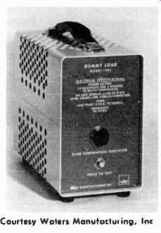
Fig. 5-6. A commercial dummy load, with 52-ohm impedance. This one is good
to 230 MHz.
Courtesy Waters Manufacturing, Inc
Turn the audio gain up on the ssb transmitter until the highest waveform like that shown in Fig. 5-6 is seen on a scope without distortion or flat-topping. An r-f voltmeter, if peak reading (as it will be if it uses a single diode), will read the voltage as indicated between the extremes of E on the pattern of Fig. 5-7. This peak amplitude is converted to rms by multiplying by .707, so the formula for reading PEP on an ssb transmitter is as follows:
_ (Epeak X .707)- PEP =-- where,
R is the impedance of the dummy load or antenna feeder.
For PEP input to the final, the plate-current meter can be used with a two-tone signal by reason of the following. With a two-tone signal the plate current will read about 64-percent of a single-tone signal on class-B amplifiers only. Multiply the plate-current meter indication by the reciprocal of .64 (or 1.57) to get the equivalent plate current, which, when multiplied by the plate-supply voltage, is the PEP power input. This method will not meet FCC requirements when you are operating at or near the 1-kW mark, nor, for that matter, does the FCC recognize a PEP figure. The FCC requirements reads something like this: "The maximum DC plate-power input to the radio-frequency tube or tubes supplying power to the antenna system of a single-sideband suppressed-carrier transmitter, as indicated by the usual plate voltmeter and plate milliammeter, shall be considered as the "input power" insofar as Sections 12.131 and 12.126(d) of the Commission's rules are concerned, provided the plate meters utilized have a time constant not in excess of approximately 0.25 second, and the linearity of the transmitter has been adjusted to prevent the generation of excessive sidebands. The "input power" shall not exceed one kilowatt on peaks as indicated by the plate meter readings." The peak meter readings based on the above will be about one half the meter reading of the plate current using the two-tone method described.
LOADING THE TRANSMITTER
When the antenna system includes an antenna tuner, all reactance can be tuned out and the load to the transmitter is a pure resistance.
When the load is a pure resistance, final plate resonance occurs at the current-dip point as indicated on the plate-current meter. In the case of an a-m rig, the plate current and voltage must not exceed the rating of the tube or tubes in the final, and coupling to the antenna should be for achieving the desired current at the plate-current dip.
Because of intermittent on-time for c-w and ssb transmitters, the final can be loaded heavier without exceeding the average dissipation rating. Higher current to the final is permissible, up to plate current saturation. Some form of output indicator should be used for fully loading a c-w or ssb transmitter. It may be an r-f ammeter, r-f voltmeter, or the forward position of an SWR meter.
For a c-w rig with antenna tuner, adjust the loading for a higher and higher plate-current at the dip, until the output indicator shows no further increase in output. Do not keep the key down for more ...
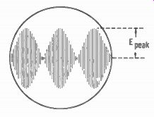
Fig. 5-7. A demodulator probe on a VTVM using a single diode will read the
peak value of an ssb signal.
... than 30 seconds at a time while making the adjustment. If your setup does not include an antenna tuner, but you arc feeding a matched (hopefully) line to the antenna, the plate-current dip is resonance only if you are perfectly matched, and the feeder-antenna load is a pure resonance. Since this seldom occurs, disregard the plate-current dip, and tune for maximum output only. If maximum output is found to be off the plate-current dip. it means the load has reactance, and the final plate capacitor is in effect, tuning out the reactance.
The foregoing is also true for an ssb transmitter. Insert a carrier to read about half the normal plate current expected. Make adjustments for loading to achieve maximum output on the output indicator. Turn the carrier up until there is no more output. The plate current times the voltage is the peak input power, and the transmitter loaded for maximum output. However, maximum ssb output under modulation is another thing. It is now necessary to establish maximum linear modulation limits, and only a scope will do this for you.
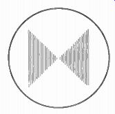
Fig. 5-8 Bow-tie pattern on scope when the ssb transmitter is modulated with
two tones (or one tone and some carrier) and audio from the speech amplifier
is applied to the horizontal amplifier of the scope.
The proper method is with a two-tone input to the microphone to form a bow-tic pattern on the scope to look like Fig. 5-8, with carrier suppressed or with one tone and carrier. Mark the limits of maximum deflection on the scope face under linear-modulation conditions.
To obtain this kind of pattern it will be necessary to pick off audio from the speech amplifier of the transmitter and couple it to the horizontal input of the scope.
Leave the scope permanently connected for voice monitoring.
While talking, never exceed the limit of the marks, and your output will be as high as it can be and still maintain linearity without flattop ping, which is important. During voice modulation, plate current will kick to about half the two-tone maximum plate current. Switch the scope to the internal horizontal sweep generator for voice monitoring.
See Section 7 for hookup details.
MODULATION MEASUREMENTS
Important to the proper operation of a phone transmitter are the amount and quality of modulation. It is desirable to know the percent of modulation, the modulator capability, the linearity, and the amount of distortion.
Modulation Percent
The laws governing amateur transmitter operation decree that the percentage of modulation should never exceed 100. nor exceed the capability of the modulator. When an a-m carrier is modulated to where the output peaks arc twice the peaks of the unmodulated carrier, it is said to be modulated 100 percent.
The best way to examine the effects of modulation is to observe the shape of modulation patterns on an oscilloscope. Any inexpensive standard oscilloscope or just a cathode-ray tube with power supply is sufficient. Since both vertical and horizontal deflection may be made directly to the deflection plates of the CRT. the tube and power to run it are all that is really needed. However, since there are a number of inexpensive scopes on the market, especially in kit form, the treatment here will assume a regular oscilloscope (Fig. 5-9). Radio-frequency output from the transmitter is coupled to the vertical-deflection plates directly. Audio from the modulator may be connected to the horizontal plates, or it may be fed into the horizontal amplifier of a standard scope.
As mentioned earlier for output measurements, a pickup loop is used to obtain some rf from the final tank. A tuned circuit will often help to supply more r-f voltage to the deflection plates. R-f can also be picked off the coaxial feeder by a Tee connection, and even a small pickup rod acting as an antenna may be used. For these latter two methods, a tuned circuit is almost certainly needed. Fig. 5-10 shows three methods for getting rf to the vertical-deflection plates of a scope CRT. In each case a tuned circuit is included. The tuned circuit can be any convenient inductor and variable-capacitor combination. which will resonate in the band being checked. The variable capacitor also can act as a level control for setting the height of the pattern on the CRT face. Fig. 5-10A shows a pickup loop consisting of a couple of turns of insulated wire, with the lead from it to the test gear twisted. Care must be exercised in coupling the loop to the final tank in the transmitter to avoid shock. In transmitters that are fully enclosed, try the Tee connection into the coaxial feeder.
This is shown in Fig. 5-10B. For non-coaxial feeders, try the pickup rod shown in Fig. 5-10C. The r-f connection is all you will need to observe wave shapes on the scope. Horizontal deflection will be obtained from the sweep circuit in the scope itself. This method is excellent if an audio generator is available to modulate the rig with a single sine-wave tone. Speech waveforms, if used, are so random that about all you can see is clipping in overmodulation in the negative direction, or flat-topping in the positive direction. It takes a pure signal tone to observe the quality of amplitude modulation.
By picking off audio from the modulator in addition to the r-f. you can produce a trapezoid pattern which may be used to observe voice modulation, thus eliminating the need for a sine-wave audio tone. A tap should be made to the high side of the secondary of the modulation transformer. Connect a 0.01 uF capacitor with a voltage rating about twice the value of the final supply. This should be followed by a string of 1-watt carbon resistors, and end with a volume control to ground. The values of the resistors should be such that the voltage from the modulator does not exceed the dissipation rating of the resistors. The hookup is shown in Fig. 5-11, and the values arc approximately right for use on a transmitter with a 1000-volt plate supply. The higher-value control is for going directly to the horizontal-deflection plates of the CRT. For feeding the horizontal amplifier of a standard scope, use about 1/100 that value. It goes without saying that good insulation is necessary between the top of the series string of resistors and any metal of the chassis or cabinet or other parts. The shunt fixed resistor across the control prevents high-voltage arcing across the wiping contacts of the control should it be dirty or loose.
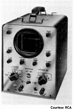
Fig. 5-9. A medium-priced oscilloscope avail able in kit form or wired. The
Model WO-33A is switchable from a medium-gain, wideband (to 5.5 MHz) amplifier
to a high-gain, medium bandwidth (to 150 kHz) amplifier. Courtesy RCA.
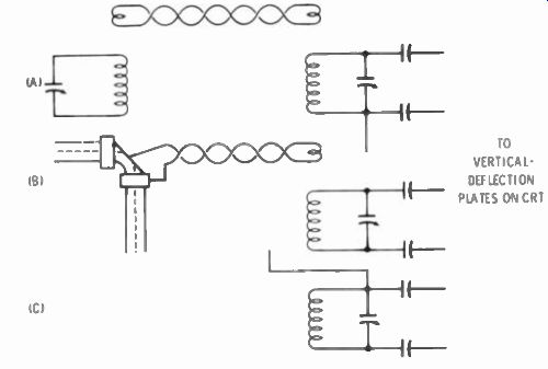
Fig. 5-10. Three methods of coupling the vertical-deflection tuned circuit
to transmitter. At A is a 2-turn pickup loop. Use the loosest coupling that
will give convenient height to the pattern. At A a slice is cut at the bend
of a right angle connector and a solder connection is made to the inner conductor
of the coax feeder. A tee connector could also be used. A 3-foot piece of stiff
wire acts as an antenna at C.
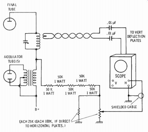
Fig. 5-11. Hookup for a trapezoid pattern from an a-m transmitter.
The modulator connection just described produces a trapezoidal pattern regardless of the type or source of the audio signal to the speech section of the modulator. Voice modulation may be used. As the modulated rf deflects the pattern up and down, the audio voltage from the modulator moves the pattern trace laterally. Modulation positive peaks correspond to highest modulated rf, and negative peaks correspond to minimum instantaneous rf. therefore the trapezoid.
To illustrate modulation percentage, both the wave envelope and trapezoid are shown together. The modulation ratio is the ratio of the difference between modulation peaks and valleys to the sum of the peaks and valleys. Fig. 5-12A shows the carrier only of an unmodulated a-m transmitter; at B is a 50-percent modulated pattern; at C is 100-percent modulation. The formula based on these patterns and the values shown in Fig. 5-12B is:
PP' - VV' Mod % = + vvl X 100
…where, PP1 is the peak-to-peak value of the crest of the modulated carrier, FF1 is the peak-to-peak value of the trough of the modulated carrier.
Another way of expressing it is the ratio of the increase in carrier modulated peaks to the carrier itself. If the peaks during modulation are twice the carrier only, it is a 100-percent increase in peak value, or 100-percent modulation.
Frequently there is a difference between the value of the positive excursion of the audio wave and the negative excursion. This may be noted by observing the deflection each side of the center horizontal reference line and the distance to the crest of the wave both above and below the center. The formula given above may be applied to half the wave height, measuring from the center line, instead of peak-to-peak. If the figures are different for upward deflection and downward deflection, modulation is not uniform, although this is not necessarily serious. It is quite common, for example, for the human voice to deflect higher in one direction than the other. Advantage can be taken of this to increase output slightly if the modulator has sufficient capability. Using voice modulation and the trapezoid-pattern system, carefully observe the shape of the top and bottom peaks and their distance from the center. Reverse the connections to one winding only of any transformer in the audio system, and make a second inspection of the shape and height of the pattern. The higher of the two, provided the peaks are clean and sharp, will give more push to your modulation without negative clipping.
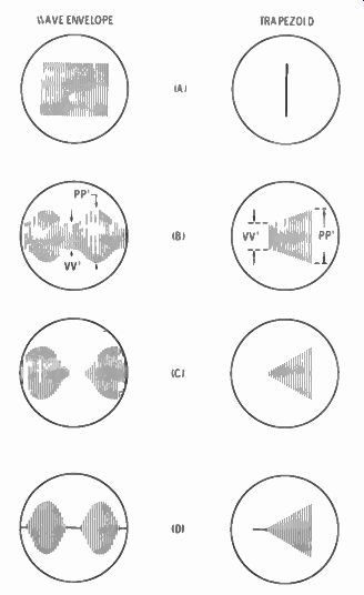
Fig. 5-12. Wave envelope (using the scope internal sweep) and trapezoid (audio
from modulator) for increasing percentages of a-m modulation. A is carrier
only. B is 50-percent modulation. C is 100-percent modulation. D is overmodulation
with negative clipping.
Negative Clipping
The most serious consequence of overmodulation is negative clip ping. When the instantaneous negative excursion of the modulating audio signal exceeds the plate supply voltage to the final r-f amplifier, there is a short duration of voltage shutoff to the final amplifier, and no carrier for that duration. This sharp break in output results in setting up very high harmonics and an interfering signal at other than the operating frequency is created. This is shown in Fig. 5-12D. Note the gaps created at the center line.
A handy circuit for monitoring an a-m transmitter for overmodulation is shown in Fig. 5-13. During the momentary bursts of over modulation resulting in negative clipping, the plate supply goes negative. If a diode is connected to the top of the modulation transformer secondary with its cathode facing the connection, current will flow during negative clipping, and no current will flow at the time the voltage is positive. Any indicator in the circuit will show the current flow while negative, thus indicating overmodulation. With the values shown in the circuit a VOM on its 10-volt DC range will kick up noticeably. The speech level should be kept down to where the VOM never kicks up. A similar circuit can be built into the transmitter using a neon bulb. A forward bias of about 65 volts must be supplied to the neon bulb to overcome the ignition voltage.
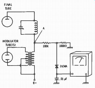
Fig. 5-13. Circuit for monitoring an a-m transmitter for negative overmodulation.
No current flows through the meter until point A becomes negative.
Modulation Capability
A plate modulator must be capable of supplying an undistorted (or nearly so) signal with power output equal to one-half the input power to the final r-f amplifier, in order to provide 100-percent modulation.
A 250-watt input to a final, for example, requires a 125-watt modulator. Without this capability the positive modulation peaks will flatten out. Not only will you not be producing the 25 percent of extra power for each sideband, but the audio will distort badly by pushing it with higher audio control settings. Any kind of distortion results in harmonics. Audio distortion produces higher-order audio tones that are not part of the intelligence requirement, but produce additional sideband frequencies higher than necessary, and so occupy a wider than-necessary bandwidth.
Here is how the power-output capability of a modulator can be measured: Determine the load impedance the final r-f amplifier presents to the modulator by dividing the plate voltage by the plate current. This should be done in order to properly match the modulator to the final anyway. Disconnect the modulator output from the final, and connect a fixed resistor of the value of plate impedance to the output of the modulator. It will take a husky-rated resistor, of course. The wattage rating would be equal to the final voltage times the current. Tap off a small portion of the output load resistor for a feed to the vertical input amplifier to your scope. Another, smaller, resistor in series at the bottom is equivalent to a tap. Connect a VOM or VTVM across the entire load resistor and set the function switch for AC volts on a high range. If the expected maximum voltage exceeds that of the highest range on the voltmeter, tap down on the resistor load, but establish a multiplying factor for voltage by noting the ratio of the tapped portion of the resistor to the total resistance.
Temporarily connect the r-f amplifier voltage feed point to the bottom of the modulation transformer secondary.
Connect an audio generator to the microphone input of the speech amplifier, and turn the attenuators down to a signal of about 10 milli volts. Set the tone for about 1000 Hz. The level of audio must not overload the speech amplifier, and should be about the right amount for the usual volume-control setting for normal transmitting modulation.
Turn everything on. Bring up the audio signal while observing the quality of the pattern on the scope. The vertical gain control will need to be readjusted on the scope as you turn up the audio in the modulator to maintain a constant pattern size for comparison. As soon as the pattern shape changes and is no longer a sine wave, back the audio down just a little. Adjust for maximum voltage reading on the output without distortion in the sine-wave. This is the point of maximum capability. Measure the voltage output on the AC meter.
The square of the voltage divided by the resistance of the load (P = E^2/R) is the power output of the modulator. If this is 50 percent or more of the power input to the r-f final, you have sufficient modulation capability.
If the power output of the modulator is below design value, check the tubes, and check all voltages. Low emission on the power tubes will limit the power output.
Other factors affecting modulation power are: low bias or excitation to the r-f final, and the final too lightly loaded to the antenna.
When the load is lightened, the input impedance to the final is higher, and the modulator will not be matched. With the audio generator connected to the input of the speech amplifier and a scope at the output, tests can also be made for clipping in the speech stages. If the output shows adequate power for modulation purposes, but the waveform is not a true sine wave, suspect clipping and attendant distortion somewhere in the modulator stages. Clipping produces harmonics, which add extra sideband frequencies and increase the band width transmitted. A search of the offending stage can be made by moving the scope input to each stage output. Use a .01-uF isolating capacitor in series with the scope lead. Move the capacitor connection from the output to the plate of the modulator driver stage, then to the next preceding stage, and so on down the line until there is no evidence of clipping. Be sure, however, that there is no overloading by having the audio generator set at too high an output. The output that just supplies 100-percent modulation is about right. Clipping shows up as a flattening of one crest of the sine wave. It is the result usually of incorrect bias on a tube, or current saturation due to a tube with low emission.
The same setup as above is useful in observing the action of speech clippers. This should be done with speech input instead of as audio generator. Observe the clipping action while talking in a normal tone of voice. Set the audio gain and clipping control so that speech at moderately low level just fills the extremes of the pattern; then high clipping will take place at loud speech levels. Clipping from a speech clipper also causes harmonics, but it is assumed that your clipper circuit also includes the necessary filters to cut off harmonics developed by the clipping action.
C-W KEYING
The oscilloscope is an excellent device for studying the keying waveform of a c-w transmitter. With output rf applied to the vertical deflection plates by one of the systems shown in Fig. 5-10. key the transmitter with dots by use of a "bug." Either an electronic or a mechanical semiautomatic key will do, but a straight hand key will not. Adjust the horizontal-sweep frequency on the scope to a slow rate to make the keying pattern stand still. It will look like one of the illustrations of Fig. 5-14. With no keying filter you should see square waveforms like Fig. 5-14A. A perfectly square wave produces an infinite number of harmonics every time the key is closed and opened. This produces off-frequency interference and is heard as key clicks. A properly designed keying filter will produce waveforms with rounded corners at the lead edge and the trailing edge. The ideal pattern is shown in Fig. 5-14B. Interfering harmonics will be reduced, and the keying will have a good sharp sound at the receiving end. Too much filtering will round the corners more, but will not have a nice, sharp make and break sound at the receiving end. At high speed, dots will tend to run together and be almost indistinguishable.
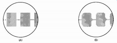
Fig. 5-14. Observing uniformly spaced c-w dots on a scope. With no keying
filter they will be perfectly rectangular as in A. Proper filtering results
in rounding the corners, which reduces key clicks, as in B.
SSB MODULATION PERCENT
Modulation percent for an ssb transmitter has no real meaning in the same sense as for an a-m transmitter. The limit of modulation on an ssb transmitter is set by the point at which flattening begins at maximum modulation. Any "percent" would be any ratio of actual modulation level to the maximum clean-signal modulation. Again, the oscilloscope pattern is the method used for seeing the modulation and measuring the height of peaks. Because voice frequencies are complex, a trapezoid pattern like that obtained from an a-m transmitter cannot be obtained from an ssb transmitter in a clean form worth evaluating. Horizontal deflection must be from the horizontal sweep circuit in the scope. Set it for a slow sweep, as you voice-modulate your ssb rig. Having established the maximum possible height by placing markers on the CRT face from output measurements. voice peaks, for maximum modulation, should just barely touch these marks on the scope. Any attempt to "hit it harder' will result in flat-topping, and splatter.
Courtesy Swan Electronics
Fig. 5-15. Transmitter mixer and driver plate coils are shown in the lower left corner of this photo of a Swan 500C. Adjustment is to the cores of the coils with an alignment tool.
TRANSMITTER ALIGNMENT
Unlike receivers, alignment of transmitters is generally rather simple. becoming a little more involved in ssb transceivers. An a-m or c-w transmitter is rather straightforward when no heterodyning stages are used. From the vfo output up to but not including the driver stage, tuned circuits are usually broad-tuned for each band. These tuned circuits are the vfo plate circuits, the multipliers, and the buffers, (unless the last buffer is also the driver to the final grid circuit). These coils are small, either chassis- or switch-mounted, and have adjustable ceramic or powdered-iron cores. Vfo oscillator coils require calibration, and driver coils are slug-tuned and are set for proper coverage with the driver variable-capacitor coverage of each band. Output adjustment was covered earlier in this section.
Begin by unsoldering the B+ from the screen or screens of the output stage if tetrodes are used. If triodes are used, disconnect the plate supply to that stage only. Connect a VTVM across the self-bias grid resistor of the output stage, or across the resistor in series with the fixed bias if that is used. Set the function and range for reading - 15 volts d-c. In this position the VTVM reads excitation to the final.
Place the vfo at midband on the 80-meter band, and the driver front-panel-tuned variable capacitor at about midscale. Using the appropriate adjusting tool (usually a plastic tool with a hex head)
adjust the vfo plate coils, and each coil from there to the output stage for a peak meter reading. Switch to the 40-metcr band and repeat this for each 40-meter coil. Do the same for each band (Fig. 5-15). For ssb transmitters put the function switch on transmit and insert some carrier.
Some ssb transceivers have a trap from grid to ground on the first r-f stage of the receiver circuit. Tuning it requires an r-f signal generator. Connect the signal generator to the antenna terminals, and set the frequency of the generator to the carrier-insertion frequency (5500 kHz in the case of a Swan 500C, for example). You should hear a beat note like that of a signal carrier. Adjust the carrier trap for minimum beat note as heard in the speaker or headphones.
VFO CALIBRATION
Calibration of the vfo is similar to that of the high-frequency oscillator of a receiver. On transceivers using a common receive transmit tuning dial, the adjustment of the receiver calibration automatically calibrates the dial for transmit (Fig. 5-16). Heterodyne frequency instruments are ideal for calibration purposes but are expensive. Heterodyne frequency meters include a built-in closely calibrated oscillator and a mixer for mixing some of the output of the transmitter with the local calibrated oscillator.
Beating the two permits adjusting the transmitter to match the oscillator standard. A much less expensive method is to use a 100-kHz crystal calibrator and a receiver. It is to be assumed, of course, that the vfo calibration is only a few kHz off frequency in order that the right 100-kHz harmonic is used. The crystal calibrator must have been previously set precisely by zero-beating with WV on a general coverage receiver.
Fig. 5-16. The vfo components are enclosed in a shield in the Swan 500C. Marked
access holes are provided to slug-tuned coils. Courtesy Swan Electronics.
The military BC 221, which was once available on the surplus market for a low price, makes an excellent moderately priced heterodyne frequency meter.
For either method above, output must be reduced by the removal of the screen voltage from the output stage or working into a dummy load, with receiver antenna shorted, if a receiver is used for the heterodyne tone.
Set the vfo for the nearest 100-kHz calibration if a 100-kHz crystal calibrator is used (or about 14 of the way in from the high end of the band), for each band to be calibrated. With the dial set for the frequency, adjust the parallel trimmer located on or near the coil until a zero beat is heard in the receiver. Move the dial to the nearest 100-kHz point (or about 14 of the way in from the low end of the band) and adjust the iron core inside the appropriate coil for zero beat. Go back to the high end and repeat the parallel-trimmer adjustment. Again adjust inductance at the low end. It may be necessary to move back and forth between the two ends several times before correct calibration is obtained. Each adjustment at one end of the dial affects the other end, but each time you go from one to the other, the calibration gets closer.
Make the adjustment for each band for which the vfo is equipped.
On some transceivers, there are only one or two bands because a band will be heterodyned for setting frequency on another. Consult your transceiver manual for a check on this. Return power to the final by reconnecting the screen of the output stage or stages, or re storing power to the plate if triodes.
SSB CARRIER ADJUSTMENT
The mechanical or crystal-lattice i-f filters used currently in ssb transmitters to attenuate one of the two sidebands are designed to pass a band of radio frequencies, the width of which is the audio frequency response. For example, the filter may have a response of 5500.3 kHz to 5503 kHz. The difference between the extremes is 2700 Hz. the planned audio frequency response. The actual response of the filter is not perfectly flat between 5500.3 kHz and 5503 kHz, but has a rolloff at the ends. The extremes of the frequency response figures are 6-dB down from the top. and the curve looks something like Fig. 5-17.
A crystal-controlled carrier oscillator of appropriate frequency beats with the audio frequencies of the voice to produce sum and difference frequencies resulting in a lower sideband, the carrier, and ...
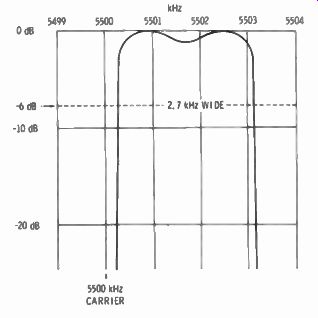
Fig. 5-17. Filter response curve of a typical ssb transceiver. The carrier
frequency is adjusted to a 6-dB drop in output with a 300-Hz modulation tone.
... an upper sideband. The carrier is balanced out, and one sideband is attenuated by the filter. The other sideband is heterodyned to the operating frequency of the band and passed on to the r-f driver stage. A small variable capacitor across the crystal in the carrier oscillator adjusts the carrier to precise frequency.
For example, if the carrier is adjusted to 5500 kHz an audio range, of 300 Hz to 3000 Hz will result in an upper sideband of 5500.3 kHz to 5503 kHz. (the bandwidth of the filter), or the sum of the audio and the carrier. If the carrier frequency is 5503.3 kHz, the lower sideband will be 5500.3 kHz to 5503 kHz, or the difference.
Adjustment of the carrier frequency is best done with an audio signal generator. Connect a variable audio signal generator to the mike input, with the generator attenuated to about normal micro phone level. Connect a dummy load to the output, and connect a VTVM with an r-f probe across the output. With the transmitter tuned up for normal operation and the audio generator set for 1000 Hz, turn up the mike gain for about normal output, and note the signal level on the VTVM. If the VTVM has a dB scale, set the signal level and VTVM range for a reading on the 0-dB mark. Now turn the signal generator down to 300 Hz. If the output has dropped 6 dB, the carrier frequency is correct; otherwise adjust the trimmer across the carrier crystal for a -6 dB reading on the VTVM. The same adjustment should be made for both the upper and lower carrier frequency if your rig has both. If yours is a transceiver, this adjustment will also be the correct one for receiving sideband signals with the recommended audio-frequency response of 300 to 3000 Hz. This is the frequency response of the example described here; it may be different for other transmitters. Consult your manual for the range of the filter and the oscillator frequency. The method of adjustment is the same.
If the design of your transceiver is such that one carrier is an exact multiple of 100 kHz (the Swan 500C has one carrier on 5500 kHz, for example), you can set it exactly to frequency by connecting a 100-kHz crystal calibrator to the antenna input and adjusting the carrier frequency to zero beat with the 100-kHz crystal calibrator on receive.
If your VTVM does not have a dB scale, select any multiple of 10 as a reference. The -6 dB point will be at 5, or half voltage.
NEUTRALIZING
In spite of excellent physical isolation between input and output of the final r-f stage, and the use of tetrodes and pentodes with good internal isolation between grid and plate, it seems that some energy from the plate gets back to the grid. When the input and output stages are tuned to the same frequency (as they usually are) any feedback will result in oscillation or some instability because of the tendency to oscillate. This feedback is positive because it is in phase.
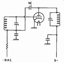
Fig. 5-18. The usual method of neutralizing a final is to capacitively couple
some output rf. out of phase, back to the grid circuit.
To overcome positive feedback it is only necessary to introduce negative feedback in the same amount. This is called neutralizing and is usually accomplished by adjusting a small capacitor of about 15 to 20 pF, which is connected between the top of the output tank coil and the bottom of the ungrounded driver coil, or final grid coil (NC in Fig. 5-18). There are several indications for lack of neutralization. The most serious is a tendency to take off by itself into self-oscillation when excitation is removed from the final r-f stage. Sometimes this occurs when the final tank capacitor is tuned slightly off the operating frequency rather than at resonance. The test is to remove excitation (only when there is protective fixed bias on the final) and tune the final tank capacitor back and forth. The plate meter should remain at zero through the full range of the tuning capacitor if the stage is perfectly neutralized. Another indication is the relation between the plate and grid currents. Normally the plate meter will dip at resonance and the grid current will increase slightly at the same time. If the grid current appears to rise slightly to one side of the plate-current dip, a recheck of neutralization is called for.
A check for neutralization involves determining how much energy gets from the grid to the plate of the output stage without benefit of amplification from the output stage. To do this remove power from the output stage by disconnecting the screen supply from the output stage if tetrodes or pentodes are used, or the plate supply if triodes are used. The screen (or plate in the case of triodes) must be bypassed to ground for both DC and rf. There should be no load attached to the output, which can be accomplished by removing the antenna connection.
Make up a simple indicator for rf like the schematic of Fig. 5-19.
This device rectifies any rf in the pickup loop and the resulting DC will show on the VOM. Couple the loop to the output tank. If high voltage is on the output tank, as in the case of tetrodes or pentodes, be very careful in coupling the loop that you do not touch the output coil with the pickup loop, unless the pickup loop is well insulated.
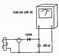
Fig. 5-19. An r-f indicator for finding parasitics. A few turns of wire on
an insulated rod will pick up rf when coupled to various points in the circuit
of the transmitter, and shows as DC on the meter.
Operate the transmitter in the usual manner except for the DC on the output. If it is an ssb rig, unbalance the carrier-balance control to insert some carrier. Bring excitation up slowly to prevent possible damage to the VOM as an output indicator.
If the output indicator meter deflects, the output stage needs adjustment for neutralization. Using a screwdriver with an insulated shaft, slowly rotate the neutralizing capacitor until there is no output shown on the indicator, as you move the output tank capacitor back and forth each side of resonance.
PARASITICS
Any piece of wire has inductance and distributed capacitance and will resonate at some frequency. Interconnecting wires in the final r-f stage of a transmitter, together with bypass or tuning capacitors, can be shock-excited into oscillation, or they can be resonant with another set of similar circuits and go into oscillation as a tptg (tuned-plate tuned-grid) oscillator. Radio-frequency chokes in both the grid and plate circuits are perhaps the worst offenders. Their inductances, together with bypass capacitors, create their own resonant circuits, which may be the same frequency in the grid and plate sides. The cure lies in changing the values of r-f choke inductance or bypass capacitors, or in swamping them with resistance either in parallel with the chokes or in series with them. Stages preceding the final, because of their lower power and usually better shielding, are not so prone to parasitics.
Unlike harmonics (which can often be easily traced because they are multiples of the operating frequency), parasitic oscillations can occur at any frequency, depending on the resonance of the offending circuit. Thus, parasitic oscillations can cause interference within an amateur band, outside the amateur bands to other services, to TV (which is the worst of all interference), and even to broadcast-band receivers. If the parasitic oscillation is near the operating frequency, it can cause instability in tuning the final. A tube carrying two frequencies can be overloaded unnecessarily, which means less power available for the signal you want to put out.
Here is how to check for parasitics: Place a short across the driver plate coil, and disconnect the antenna. Put a lamp in series with the 120-volt input to the transmitter to prevent overdissipation in case the plate current runs away. If the final has fixed bias replace it with a grid-leak resistor of about 10K to 20K. Turn the transmitter on, and revolve the final tuning capacitor. If there is any kick in the plate meter you have parasitic oscillation.
If there is an increase in plate current, leave the capacitor set at the point where the increase occurs and couple a grid-dip oscillator, switched to be an absorption wavemeter, to the output (CAREFUL! HIGH VOLTAGE). Go through the entire set of GDO coils and tune across each coil band and watch for an upward kick of the GDO meter. When the meter kicks up. this is the frequency of parasitic oscillation. If there is no indication from the output tank, try coupling the GDO to other wires in the final, both input and output. When the frequency of oscillation is found, turn the transmitter off and, using the GDO as a grid-dip oscillator, couple to all circuits in the final until you find one resonating at or near the frequency found by the absorption wavemeter method. You may find one in the output and one in the input near each other in frequency.
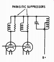
Fig. 5-20. Parallel a 1-mH choke with a 100-ohm resistor to make a parasitic
suppressor. A 2-watt 100-ohm carbon resistor with about 10 turns of heavy wire
wound over it and connected in parallel is often a good suppressor.
PARASITIC SUPPRESSORS
Be particularly suspicious of r-f chokes. Check their resonant frequency with the GDO. If resonance is in one of the TV bands, replace the choke or chokes with other values. Parasitics are also cured by changing the length of wires, preferably shortening them where possible, or by introducing parasitic suppressors. A parasitic suppressor is an r-f choke with a resistor across it or in series with it. Fig. 5-20 shows the circuit for the most popular type.
Another method for checking for parasitics and determining their frequency is to couple the GDO into the driver coil with the driver plate tuning capacitor disconnected. Pull out the driver tube. (The GDO becomes the excitation to the final.) The rest of the setup is as described previously. Tune the GDO through all of its frequencies. If plate meter kicks up, that is the frequency of the parasitic. With the transmitter off use the GDO set for the same frequency that caused the kick, and go searching for the circuit resonating at the frequency.
CLASS-C OPERATION
The final r-f stage for c-w and a-m phone is operated at twice cutoff for bias and is called class C. The object in adjustments is to attempt to get the most out for the DC input without exceeding the rated dissipation. This is done by loading, and differs whether it is for c-w intermittent service or a-m phone continuous-carrier service.
The object is to achieve as near the maximum theoretical efficiency of 75 percent as possible. Linear plate modulation of a class-C amplifier depends on matching the impedance and having a modulator with sufficient power capability.
CLASS-B LINEARITY
When modulation occurs ahead of the final r-f stage, then the final must have linear amplification characteristics; that is, the output must be a duplicate of the input, at greater power. In audio amplification this is achieved by properly designed single-ended or push-pull class-A; or by push-pull class-AB,. class-AB,, or class-B amplifiers.
These classes differ as to the amount of grid bias used, and whether or not the grids are driven positive at times. The latter three types must be used in push-pull to cancel even-order harmonics in audio amplifiers. The most efficient of these is class-B, with the bias at or near the cutoff point. At cutoff the no-signal plate current is nearly zero, and plate-current flow is intermittent. Thus the stage can be more heavily loaded without exceeding its dissipation rating.
Linear r-f power stages are operated in class-B bias conditions.
Because of the flywheel effect of the output tank, only one tube need be used, push-pull operation not being necessary. A previous stage may be amplitude-modulated (although this is not usually done, be cause you are ahead in a-m phone operation with plate modulation of the final). Class-B amplifiers are used, almost exclusively, for ssb transmission.
If a class-B stage is not operated properly it will not be a linear amplifier. Nonlinearity produces distortion, both harmonic and inter modulation. Intermodulation distortion results in sum and difference products of frequencies beating with each other and producing other frequencies. Here is an example to illustrate this: Modulate a 3.9 MHz signal with two audio frequencies, 3000 Hz and 4000 Hz. With the carrier suppressed, the transmitted sidebands will produce radio frequency signals of 3.897 MHz and 3.896 MHz (lower sideband). Harmonic distortion will double the 3.897-MHz signal to 7.794 MHz. Intermodulation distortion will beat the 7.794-MHz signal with the 3.896-MHz signal producing a new signal at 3.898 MHz. At voice frequencies the harmonics of any frequency will beat with any other frequency to produce new signals. This is transmitted as side band splatter and gives rise to interference to other stations.
The only way to properly adjust a class-B amplifier for linearity is by the use of an oscilloscope. In addition to a scope a two-tone audio source is most helpful, but a single tone plus some carrier can be used. The human voice cannot be used.

Fig. 5-21. A bow-tie pattern on a scope from the two-tone (or one-tone and
carrier) test method. Sharp corners, and a perfect X outline means good linearity,
without flat-topping.
Using a dummy load, couple the vertical plates of the CRT of the scope to the output using one of the methods described before.
Couple the output of the speech amplifier to the horizontal input of the scope. With the transmitter tuned for normal voice operation apply sine-wave audio to the microphone input (a tone of about 3000 Hz and one about 4000 Hz). The output of two variable-frequency audio generators can be paralleled, with the signal level from each equal. Turn up the microphone gain on the transceiver and observe the pattern of the scope. It will be a bow-tie pattern like Fig. 5-21.
Now turn up the microphone gain to the point just before the top and bottom peaks on the bow-tie lose their sharpness. At this point you are at maximum output just before flat-topping. The signal must not be held there for more than about 30 seconds at a time. One easy method of observing the maximum signal trace without over dissipation is to insert a semiautomatic key into the key jack and key a series of fast dots. This provides an intermittent signal for observation. The pattern may flicker but you can see what is happening at maximum output without worrying about overdissipation.
Rounded top and bottom corners indicate flat-topping. Flat-top ping can result from three things: under-coupling to the antenna, over excitation from the r-f driver, or too high a speech level (the most common reason). Increase antenna loading as you observe the pat tern. If the flattening does not clear up, you were previously loaded enough, and probably you are just overdriving the input to the amplifier by too much rf or audio. The crossover point between the two parts of the bow-tie should be a perfect X. If there is a tapering at the points, it is usually a sign of too much bias. Adjust the bias for a perfect X at the same time not exceeding the recommended resting current to the plate with no modulation. Observe the sides of the pattern. They should be straight lines. If all voltages to the final are correct and antenna loading is the right amount, the sides will be straight and the stage will be operating in a linear manner.