Whether it is a complete receiver alone, or the receiver portion of a transceiver, measurement of receiver performance is desirable either in part or complete. Important performance characteristics of a receiver are sensitivity, selectivity, image response, calibration accuracy, and sometimes input impedance and noise factor.
Sensitivity is the receiver's ability to amplify weak signals. The limit of sensitivity is external and internal noise, which masks weak signals no matter how much gain the receiver may have. This is referred to as the S/N Ratio, or signal-to-noise ratio. A more accurate designation is S + S/N or signal plus signal-to-noise ratio. Overall gain of a receiver is stated in microvolts (millionths of a volt) signal input that produces a given audio output-usually one-half watt. But a receiver with high gain can lose its value in on-the-air performance if the internal noise is high and masks weak signals. Both the S + S/N ratio and gain are important in evaluating a receiver's ability to perform on weak signals. Communications receiver sensitivity is expressed in micro volts of r-f input to produce a signal 10 dB above the receiver internal noise. Selectivity is the ability of the receiver to separate signals so the desired signal stands out from all others. Selectivity is expressed in a bandwidth in kHz, which represents a band of frequencies, the end frequencies of which are 6 dB down from the center frequency. When a signal is 6 dB down it is received at half the power it would be as compared to when tuned on-the-nose. High selectivity (about 0.5 kHz) is desirable for c-w signals; wider selectivity is necessary (about 3 to 5 kHz) for phone signals. Too high selectivity on phone clips the sidebands and affects intelligibility.
Image response is the ratio of sensitivity to the signal being tuned to the sensitivity to the image of that signal. An image of the signal can be heard at twice the intermediate frequency above or below the signal frequency, depending on whether the high-frequency oscillator of the receiver is above or below the signal frequency. Image response is affected by the selectivity of the "front end," or those stages which tune the signal frequency and which precede the i-f stages. Poor image response can result in interference from another signal twice the intermediate frequency away, if it is a strong signal.
Calibration is the ability to read the received frequency accurately on the calibrated tuning dial. It is expressed in percent of the dial reading and is a function of the accuracy with which the high-frequency oscillator tracks with dial calibrations.
Input impedance is the load in ohms the receiver input reflects to the antenna feeder as a source of signal. When the load impedance is equal to the source impedance, best transfer of power is accomplished in any electrical system. No receiver has a constant and perfect load impedance clear across each band. Input-impedance matching on receivers is a matter of good design, but a reasonable mismatch should not be taken seriously. It has little effect on overall performance. Published figures represent sort of an average across the band, on each band.
Noise figure has to do with noise generated internally in a receiver. It is expressed by the letters "NF" and is given as so many dB above a theoretically perfect noise-free receiver. Internal noise is greatest in the mixer stage and is primarily due to "shot effect," which is the random irregularity of electron flow. Good preamplification overrides mixer noise. Noise can originate in preamplifier stages and in tuned circuits, and dielectric resistance leakage in components and transit time in tubes produce noise. The higher the frequency of the tuned circuits is, the higher is the noise. In addition, the motion of molecules in tuned circuits produces thermal agitation noise and is related to temperature.
MEASURING INSTRUMENTS
Instruments are important to measurement, of course. Some are elaborate, and some are simple enough to build yourself.
The most important instrument for work on a receiver is the signal generator. Basic signal generators consist of a high-frequency oscillator, an a-m modulator, sometimes a buffer stage, and, of course, the power supply to power this instrument. All include an attenuator of some sort, and some have an r-f voltmeter connected to the output, and preceding the attenuator.
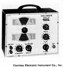
Courtesy Electronic Instrument Co., Inc.
Fig. 4-1. The Eico Model 324-K signal generator has output from 150 kHz to 145 MHz on fundamentals. The built-in 400-Hz modulator is variable up to 50 percent.
Quality varies considerably in signal generators. Better instruments will have more stable oscillators with more accurate calibration of the tuning dial. Wide frequency coverage is achieved in the same way as in receivers, by bandswitching (Fig. 4-1). An audio oscillator modulates the r-f oscillator. Inexpensive units have only one audio frequency (usually about 400 Hz) and the percent of modulation is about 30 percent. Better instruments may have a variable-frequency audio oscillator and provide up to 100-percent modulation by modulating a later stage. For amateur measurements, a single audio frequency with 30-percent modulation is usually sufficient. When the built-in r-f voltmeter is employed, the instrument is better known as a Microvolter. Any good external VTVM with high r-f response can be used to set the initial reference output voltage, however. Other factors affect quality and therefore usability. Good r-f shielding is essential to prevent r-f leakage from the internal circuitry to the receiver in order to be able to read low signal levels more accurately. A well-designed step attenuator will have a minimum of stray capacitance in order to maintain accuracy of attenuation at the higher frequencies, and be itself well shielded. The power supply should be regulated to prevent line-voltage fluctuations from affecting the frequency of the oscillator.
A sweep generator (Fig. 4-2) is something like a signal generator, but with some important differences. The amplitude modulator is eliminated. The high-frequency oscillator is made to sweep across a band of frequencies at a regular rate. The sweep generator must be ...
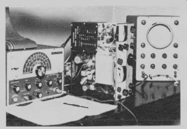
Fig. 4-2. A sweep generator and scope connected to an amateur transceiver.
The trace of Fig 4-3 is an actual photograph of the selectivity curve obtained
from this hookup.
... used with an oscilloscope. When the generator sweep rate is synchronized with the horizontal sweep on the oscilloscope, the scope pattern becomes a visual picture of the selectivity response of the receiver to the frequencies being swept. Sweeping the frequency means that the oscillator frequency is changing constantly over a range of frequencies.
For example the oscillator can be set for a center frequency of 7.4 MHz and swept over a range of from 7.35 MHz to 7.45 MHz. If the receiver is tuned to 7.4 MHz. the scope will show the highest vertical deflection to be at 7.4 MHz. and the lower amplitudes on each side, indicating the attenuation of frequencies below and above 7.4 MHz.
This is seen on the scope as a curve like the one shown in Fig. 4-3, which is called the selectivity curve of the receiver.
A number of methods are used to sweep the high-frequency oscillator. The oldest uses a variable capacitor, the rotor of which is attached to a motor. The motor spins the rotor of the capacitor. The capacitor is in the high-frequency oscillator circuit. With its constantly changing capacity there is a constantly changing frequency. At least one generator uses a powdered-iron slug attached to the voice coil of a speaker. The speaker is made to vibrate at a 60-Hz rate from the power-line frequency, thus causing the slug to move in and out of an inductor, which is part of the high-frequency oscillator circuit. A currently common method used in inexpensive sweep generators uses a saturable reactor. The band coils of the oscillator, either as separate coils or as taps on a common coil, are wound on a powdered-iron core.
Also on the core is a winding of heavy wire. A varying rate of direct current is passed through this extra winding. At high current the core ...
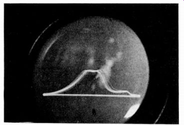
Fig. 4-3. Selectivity curve as shown on the scope face.
... of the inductor saturates, and the inductance is lowered. At lower current, the inductance increases. As the inductance is made to change, the oscillator frequency changes in step with the scope horizontal sweep. A fourth method uses either a variable-reactance tube circuit, or a varicap which is a solid-state diode whose internal capacitance changes with varying direct current through it. These act as variable capacitors in the oscillator circuit. These last two methods are electronic. In these methods the variable voltage is obtained from a saw tooth oscillator which provides a sweep linearly from one frequency to another, then a quick return to the first frequency.
An oscilloscope (Fig. 4-4) must be used with a sweep generator. An oscilloscope is also important in observing audio distortion and audio frequency response in speech amplifiers and modulators. Since transmitter modulators are intentionally limited in frequency response, and a small amount of distortion is tolerable, measuring the response and distortion only satisfies one's curiosity. A scope may be considered an inertialess VTVM. The beam of the cathode-ray tube is deflected without inertia and is therefore almost instantaneous. The deflection plates of the CRT in the scope take several volts to deflect the electron beam, therefore they are preceded by amplifiers, one for vertical deflection and one for horizontal deflection. Quality and price of a scope are based on size of the CRT, gain and bandwidth of the amplifiers, and variety of functions. Even the most inexpensive scope is adequate for most amateur needs. A modification of the oscilloscope is used to monitor the modulation of transmitters. This will be described in greater detail in a later section.
A crystal calibrator (see Section 7) is a crystal-controlled oscillator that produces accurate signals for pickup in the receiver. The ...
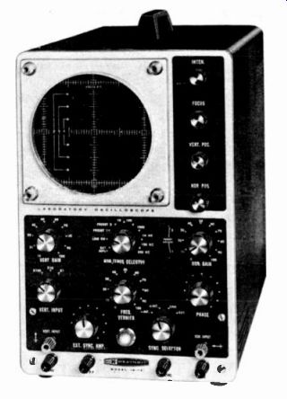
Courtesy Heath Co.
Fig. 4-4. A wide-band oscilloscope which can be built from a kit. The vertical amplifier sensitivity is 0.025 V/inch deflection, and has a response of ± 1 dB from 8 Hz to 2.5 MHz.
... simplest consists of a 100-kHz crystal in a single tube or transistor oscillator, designed to be rich in harmonics. When coupled to a receiver. a signal will be heard every 100 kHz as far up in frequency as 30 MHz. A small variable capacitor in the crystal circuit allows adjusting the frequency to beat with WWV as a standard, thus providing extremely accurate frequency spots. A simple 100-kHz crystal calibrator should be permanently connected to your receiver for a quick check of the dial frequency every time you use it. Better crystal calibrators include multivibrator stages, one set to oscillate at 10 kHz, and often one oscillating at 1 kHz. These lock in with the 100-kHz oscillator for accurate 10- and 1-kHz spots. Some calibrators start with a 1-MHz crystal and include multivibrator circuits to give outputs every 1 MHz, 100 kHz, 10 kHz and 1 kHz. Each can be heard separately by switching.
Noise generators are just what the name implies. The shot effect of a solid-state or vacuum-tube diode produces a random-frequency output which covers the entire useful amateur range. They are excellent for peak-aligning the front end of a receiver. Tracking of r-f stages in a receiver is easy with a noise generator. It is only necessary to peak trimmers and coil slugs for maximum noise in the output of the receiver. An easy-to-build noise generator uses a solid-state diode. A more elaborate one, and one that can be used to make actual S + S/N measurements, uses a 5722 vacuum-tube diode which is designed to produce a measured amount of noise. Circuits for both are given later in this section.
The grid-dip oscillator (GDO) should be the number-two instrument in the ham shack, next to a VOM or VTVM. Among its many uses is that of a signal generator. It is too unstable and inaccurate for precision frequency measurements, but it does produce tunable signals for rough calibration and for alignment. It is an excellent instrument for receiver design use, in that it may be used to set all tuned circuits very near the proper frequency while cold, that is, with no power applied to the receiver.
MEASURING SENSITIVITY
Overall sensitivity is expressed as the signal level required to produce a certain amount of audio power in the output (usually one-half watt) or the signal level required to overcome the internal noise.
The latter is used more frequently for ham-type receivers, and is the signal input needed to produce an output of 10 dB above the internal noise. A common specification may read: Sensitivity -- 1uV for 10 dB S/N. This means 1-microvolt, 30-percent amplitude-modulated signal will be heard in the output, 10 dB above the internal noise.
It must be kept in mind that sensitivity figures published in the literature or in catalogs attempt to show the best figures, and so apply to measurements made on the lowest band. Sensitivity is hardly ever the same across any one entire band or on each different band of a receiver. Since receiver noise increases at higher frequencies, and circuit Q's are lower, it would be a mighty difficult feat to engineer the same high sensitivity into the higher bands as the lower.
It takes a good signal generator or micro-volter to make meaningful sensitivity measurements on a high-gain ham receiver. The signal generator must be well shielded, and it must have a good step attenuator. For signal outputs down around 0.5 to 1 microvolt, all of the signal must come from the output jack and be properly stepped down from the attenuator. With poor shielding, your attenuator may read 1 microvolt, but the actual signal may be much more, either from direct radiation from the instrument or around the attenuator network to the output jack. The higher the frequency is the more critical r-f leakage becomes.
In addition to the signal generator you will need a VOM or VTVM for making output readings. It is connected to the output across a resistor which replaces the speaker. The VOM or VTVM must be sensitive enough to read the internal noise of the receiver on its AC or output function. A speaker is an inductive load to the receiver output and is, there fore, frequency sensitive. That is, voltage readings across the speaker may be different for different audio frequencies of the same level.
The voltage reading of random noise may be different from that of a 400-Hz audio tone, for example. Therefore, output measurements are made across a resistance of the same impedance value as the speaker substituted for the speaker.
SENSITIVITY HOOKUP
Temporarily disconnect one leg of the speaker from the amplifier output, and connect a 3.5- or 4-ohm resistor across the output. If your receiver has a 500-ohm line output, so much the better. Disconnect the speaker and connect a 500-ohm resistor across the 500 ohm output. Set the VOM or VTVM to the AC or output function, and connect it across the resistor. If the resistor is a 3.5- to 4-ohm resistor, you will need to use the most sensitive range; if the output is 500 ohms, a higher range setting may do. Unless the VOM or VTVM has a very low, low-range scale, the speaker output may not have enough voltage to give a good reading. In this case, connect the VOM or VTVM across the primary of the output transformer.
Fig. 4-5 is the hookup for measuring sensitivity. Connect the signal generator to the input of your receiver with shielded cable.
Most signal generators have a 50-ohm termination at the end of the output cable. If you operate your receiver from a 50-ohm coaxial antenna feeder, connect the generator output cable directly to the antenna input of the receiver. If you normally operate your receiver from a random length of wire for an antenna, a dummy-antenna network must be connected between the output of the generator and the receiver. A dummy-antenna is easy to make, the schematic is shown in Fig. 4-6. Keep leads as short as possible and enclose the network in a metal box-it must be well shielded to prevent stray pickup. Turn on the receiver with the r-f sensitivity control at maximum and bandswitch on the lowest band. If the measurement is to be made...
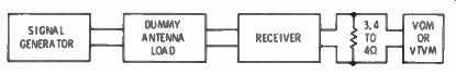
Fig. 4-5. Hookup for sensitivity measurement. If you operate your receiver
from a 50-ohm feeder, omit the dummy-antenna network.
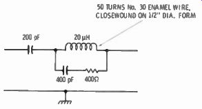
Fig. 4-6. This dummy-antenna network acts like a random length antenna. Use
it between the signal generator and receiver input.
...on the basis of input microvolts versus audio power out, the audio volume control must also be at maximum. If the measurement is to be made for dB above the noise, the setting of the audio volume control is not important, since very little noise is created in the audio stages. Be sure the receiver is not tuned to a strong signal by plugging in the headphones and listening. You should hear only noise as a rushing sound. Between the audio volume control and range switch on the VOM or VTVM, make adjustments so the noise reads 0 (zero) dB on the meter scale. You are now set up for a beginning reference point.
It is best to stabilize the signal generator by turning it on about one-half hour before measurements are made. Set it up for 30-percent internal modulation. Adjust the tuning dial and band to the frequency of the receiver. If the signal generator has a built-in reference r-f voltmeter, adjust the variable-output control for a 0.1-volt reading on the meter. If it does not have a built-in meter, disconnect the generator from the receiver, transfer your VTVM (a VOM won't do here) adjusted to read 0.1 r-f volt to the output of the generator.
With the step attenuator for minimum attenuation or maximum output, adjust the variable control for 0.1-volt indication on the VTVM. Reconnect the VTVM to the output of the receiver, and the signal generator to the receiver input. Do not touch the variable control on the signal generator; adjustments of output level must be made with the step attenuator, until the end of the test when the variable control may need to be used.
The step attenuator may be calibrated in dB. It must be translated to output in microvolts. Set at zero-dB attenuation, the output is 0.1 r-f volt. At 20 dB, the output is 1/10 of 0.1 volt, or .01 volt. At 40 dB, divide by 10 again (which equals .001 volt) and so on down the line. For each 20-dB position of the switch, move the decimal point to the left one digit. At 100-dB down, the output will be 1 microvolt (uV). For readings between 0.1 /uV and 1 /uV. and between 1 /uV and 10 /uV, adjustments will be made with the variable control for multiplying factor.
With the attenuator set at 60 or 80 dB. rock the tuning control on the signal generator for maximum reading on the output VOM or VTVM. If the reading is off scale, move the attenuator down another 20 dB. Set the attenuator for the nearest reading on the VOM or VTVM to 10 dB above the zero-noise reference point. Should the nearest setting be, for example, 8 dB, then turn the variable control on the generator up to where the output meter on the receiver reads 10 dB above 0. The voltage reading on the signal-generator output meter will be the multiplying factor for voltage output above 1 uV; in this case 1.5 /uV, which means that the sensitivity of the receiver is 1.5 /uV for 10 dB S/N. If the receiver output meter reads, for example, 13 dB, reduce the variable control on the generator to the 10-dB point on the receiver output meter, and multiply the 1 uV reference by the generator meter reading. In this case a reading of 0.7 /uV on the generator would bring the output meter down to 10 dB, and the sensitivity of the receiver would be 0.7 /uV for 10 dB S/N. A rating in dB is an expression of power ratio and is based on the formula:
dB = 10 log P_in / P_out
Every 10 dB represents a 10-times change in power ratio. Since, in Ohm's law power varies as the square of voltage, voltage ratios expressed in dB are based on the formula:
dB = 20 log E_out/E_in
For every 20-dB change in voltage there is a 10-times change in voltage ratio. Many less expensive signal generators have their step attenuators marked in ratio of voltage output, such as X 0.1 x .01 etc. These provide a direct ratio of generator reference voltage to its output.
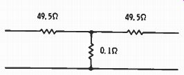
Fig. 4-7. A 60-dB attenuator made of to three resistors.
In a number of medium-priced generators the output step attenuator will not go down as low as 1 /uV. The output of these generators at minimum is much too high to measure a good communications receiver, but they can be used with an external fixed attenuator. Fig. 4-7 is the schematic of a 60-dB attenuator which may be connected between the output of the signal generator and the input to the receiver, and will divide the generator output by another 1000. Sensitivity measurement based on power output is more like an overall gain measurement, disregarding internal noise. The setup is like the foregoing dB measurement but without the use of zero-dB noise-reference reading on the VOM or VTVM output meter. Instead it is based on the modulated signal required at the input to produce a certain power level (usually 0.5 watt) at the receiver output.
The hookup is the same as before. Adjust the signal-generator output to produce 0.5 watt of audio power in the output. In this measurement, the audio volume control must be at maximum. Since the reading is in volts, the selected voltage must be related to the power using Ohm's law:
or.
Assuming a 4-ohm resistor and solving for E at 0.5-watt output:
E = __/ 4 X .5
= __/ (2.0)
= 1.4 volts where,
P equals output power in watts.
E equals voltage across the load resistor.
R equals the resistance of the load.
Adjust the signal generator to produce 1.4 volts output. The r-f volt age into the receiver is the sensitivity of the receiver using this method.
STAGE-BY-STAGE GAIN
If you have checked your receiver for sensitivity and found it wanting, you will be curious to know where the trouble is. A stage by-stage gain measurement may be made which may reveal one stage in trouble. If the zero-dB noise reference can be established, but the sensitivity figure is way below what it ought to be, the trouble is probably in the front end, or r-f stages. If no noise is measurable, or is barely heard with gain wide open in a normally sensitive receiver. gain has been lost in the i-f or audio stages.
Most signal generators have a jack for using the 400-Hz modulator externally. Connect this to the high side of the audio volume control or across the second-detector load resistor. An audio signal of 0.5 to 1 volt in should produce the rated power output. The output should be measured across a dummy-load resistor replacing the speaker as described before. If. for example, the output is rated at 1 watt, a voltage of 2 volts across the resistor should be obtained with the 0.5 to 1-volt input to the audio stages. Again, Ohm's law is used:
E = __/ RP, or E = __/ (4 X 1)
... or 2 volts, if a 4-ohm dummy-load resistor is used.
A modulated r-f signal is used to measure the gain of i-f and r-f stages. Connect your VTVM across the second-detector load resistor and set the VTVM function to read DC on the 1-volt range. Connect the signal generator to the primary of the last i-f transformer and adjust the variable control on the generator for a 0.1-volt reading on the VTVM. The signal generator should be set at the intermediate frequency of the receiver (or approximately so) to begin with. Single sideband (ssb) receivers do not have a second-detector load resistor.
In that case, make connection to the secondary of the last i-f trans former, or to the grid of the tube or base of the transistor which follows.
On ssb receivers you must kill the bfo (or carrier-injection signal) by pulling out the tube if the receiver is a vacuum-tube receiver, or by shorting the oscillator coil if the receiver is a transistor receiver.
A demodulator probe must be used on the VTVM or VOM to convert the modulated-rf to audio. Fig. 2-30 in Section 2 is the schematic of a simple demodulator probe you can make if necessary.
Move the signal generator output cable to the grid of the last i-f tube, or the base of the last i-f transistor. Turn the signal-generator attenuator down until you get the same reading (0.1 volt) on the VOM or VTVM. The difference in reading is the gain of the stage.
If the attenuator is marked in decimal dividers, the gain is a direct reading with in-between attenuator range readings taken by adjusting the variable control. If the attenuator is marked in dB, the terms must be converted to gain as a direct ratio, although some gain measurements are made in dB. Since the gain is in voltage rather than power, interpreting dB to ratio means there is a voltage gain of 10 for each 20 dB. Move the signal generator output cable to the next preceding i-f stage and make a gain measurement. The added attenuation required to reduce the output is the gain of that next preceding stage in dB. For voltage gain ratio, divide the overall gain of both stages by the gain of the last stage, to get the gain ratio of the stage alone.
When moving the signal generator from stage to stage it is important that the output leads are dc-isolated to prevent shorting the stage inputs. Check between hot terminal and ground with a VOM on ohms. If there is continuity, use a .01uF capacitor in series with the hot lead of the signal generator. An isolating capacitor is not necessary at the receiver antenna input.
Continue on down the line with each stage from right to left (as viewed on a schematic) until the antenna terminals are reached.
Intermediate-frequency stages have very high gain because of the very high Q of the i-f coils-gains of several hundred are possible.
The converter stage usually has little gain, perhaps only about 10 or less, because they are designed for best conversion efficiency rather than gain. R-f stages, too, have much lower gain than i-f stages, be cause of the relatively poor Q of the tuned circuits. A receiver fault is found by noticing a substantial difference between two similar stages. If you find this is not so. then suspect rather bad misalignment, which we will discuss later.
Stage gain is the voltage ratio between output and input:
Gain (G) = E_out / E_in
MEASURING SELECTIVITY
The selectivity of a receiver may be measured, or a curve plotted, by the same signal generator described before. In fact it need not be as good a signal generator. The most important quality the signal generator must have is good bandspread on the dial, and a tuning mechanism with no backlash. It is important to be able to read small frequency changes each side of a center frequency.
A sweep generator and oscilloscope are ideally suited to measuring selectivity, while at the same time observing the shape of the selectivity curve. This setup is a great time saver when making adjustments to the tuned circuits- you see what happens as the adjustments are made. An auxiliary variable-frequency signal generator or crystal calibrator is also necessary to properly use a sweep generator. It adds small pips to the curve on the scope screen to establish reference points, and is called a marker generator.
While some selectivity is contributed by a well-designed front end in a receiver, nearly all meaningful selectivity is in the i-f stages. Signal frequencies are converted to a single intermediate frequency for the very reason that at one lower frequency, circuit Q is much higher. While overall selectivity can be measured by connecting the signal generator to the antenna terminals, it is easier to make the measurement at the intermediate frequency, and the results are practically the same.
THE SELECTIVITY HOOKUP
To make proper selectivity measurements it is necessary to make a couple of minor operations on the receiver. Because avc action affects measurement results, it will be necessary to kill the avc. With the bottom plate of the receiver off, and the receiver turned on but with no signal tuned in. measure the fixed bias in the avc line with a VTVM. Parallel this fixed bias with an external voltage source of the same value. The easiest method is to connect some flashlight cells in series, and connect the string across the avc line, making sure the polarity is the same as the original. If, for example, you have measured - 3 volts of fixed bias on the avc line, two flashlight cells in series will do. The low internal resistance of the cells will prevent an increase in bias when a signal is applied, and a fixed-bias value of - 3 volts will be retained. The second operation is to kill the high frequency oscillator, since it may beat with the signal generator and show false signals. In a vacuum-tube receiver pull out the h-f oscillator tube. If the tube is multi-purpose, or if the receiver is transistorized, you can kill oscillation by inserting a piece of wire or metal foil between the plates of the oscillator section of the tuning-capacitor gang. Be careful not to be bend the plates-insert metal just enough to short the rotor and stator plates of the capacitor.
Connect a VTVM across the diode load resistor in the second detector with the function switch to read DC voltage, or connect a VOM or VTVM across the speaker terminals with the function switch set to read AC volts. Ssb receivers with a product detector only do not have a second-detector diode necessary to convert the r-f signal to audio for measurement by the VTVM. In this case it is necessary to provide a diode detector by using a demodulator probe on the VTVM.
A connection must be made between the signal generator and the input of the converter stage. If the receiver uses vacuum tubes one of the easiest methods is to lift the shield from the converter tube from above the grounding tabs and clip the hot lead of the signal generator to the shield and the ground lead to the chassis. This provides capacitive coupling to the elements of the converter tube. On a transistorized receiver clip the hot lead to the base of the converter transistor. Tune the signal generator to the intermediate frequency, and set the function for r-f output only if the VTVM is across the diode load resistor, or set to 400-Hz modulated-rf if a VOM or VTVM is connected to the output. The hookup is shown in Fig. 4-8.
In a dual-conversion receiver the generator should be connected to the first converter which follows the preamplifier stage or stages.
While the higher intermediate frequency of a dual-conversion receiver is used to reduce image response, it does add to selectivity as well, and should be included in an overall selectivity measurement.
With the receiver on and the r-f sensitivity control full on, adjust the frequency of the signal generator for maximum deflection on the ...
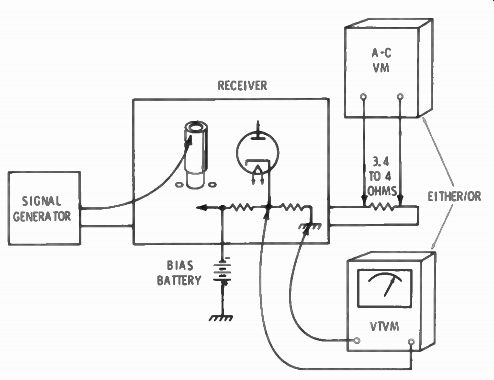
Fig. 4-8. Hookup for checking selectivity. The lifted converter-tube shield
provides capacitive coupling to the plate of the tube.
... meter. Keep the level of the signal generator as low as possible, and yet get a good deflection on the meter. An overloaded receiver will give erroneous results. Adjust the level of the signal generator to give zero-dB reading on the dB scale of the meter. Carefully note the exact frequency at which peak output is obtained. Slowly move the signal generator tuning dial above the peak frequency until the meter reads - 6dB, and note the frequency. Do the same below peak frequency. Subtract the lower frequency from the higher frequency, and the difference is the bandwidth of the receiver at the 6-dB points.
For example, the receiver has a 455 kHz i-f. Peak output on the VOM or VTVM occurs when the signal generator is tuned to 455 kHz. As we move the signal generator dial down and watch the meter, the - 6dB point is reached when the signal generator dial reads 453.5 kHz. Moving the tuning dial up in frequency, the meter needle rises again to the zero-dB point and drops again above 455 kHz. It reads -6dB at 456.5 kHz. The 6-dB points are, therefore, 453.5 kHz and 456.5 kHz, and the difference between the two is 3 kHz, which is the bandwidth of this receiver at the 6-dB points.
Selectivity figures are sometimes also given for points at 50-dB down. The method of measuring is the same as for the 6-dB points except the frequency extremes are observed for a meter drop to 50 dB below the zero point both above and below the center frequency.
If, in the foregoing example, the bandwidth were 30 kHz at the 50-dB points, it would indicate a good receiver for phone reception.
A selectivity curve can be plotted using a signal generator. The method is as described above, except that dB figures are plotted against frequency over a wider range below and above the center frequency. In the previous example, begin by setting for zero dB at the center frequency, then move the signal generator down to about 440 kHz, and chart dB against frequency for each kHz up to about 470 kHz. The chart may look something like this:
CENTER FREQUENCY IS 455 kHz
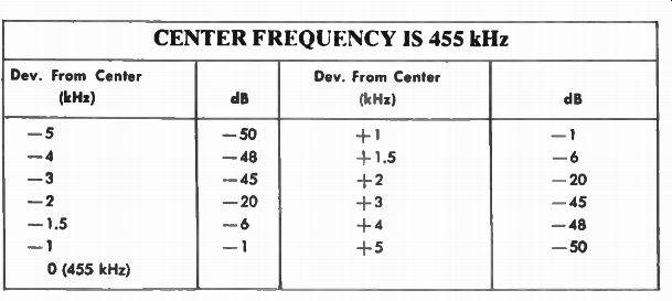
The next step is to convert this to ruled paper to see the selectivity curve. Fig. 4-9 is a selectivity curve based on the figures above. Note that this is in dB which is a logarithmic method of expressing a ratio. Since our output meter measures in volts, basically, the dB scale on it follows the ratio dB = 20 log E1/E2. If your meter does not have a dB scale you will need to convert volts to dB using this formula. The right hand Y axis of Fig. 4-9 shows the voltage ratio and how it relates to the logarithmic ratio.
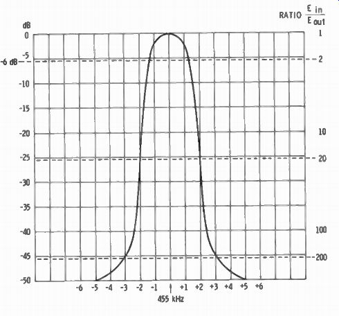
Fig. 4-9. A receiver selectivity curve plotted from the figures tabulated
in the text.
On a selective receiver it is often not possible to reach the lower dB outputs by detuning the signal generator. At a bandwidth of 10 kHz, the output meter may appear not to read anything. In such cases a reverse method may be used. As you tune this signal off center frequency, increase the output of the signal generator to maintain a zero-dB reading on the output reading. Plot the amount of increased output in dB or voltage ratio required of the signal generator to maintain the zero reference, using the step attenuator. An advantage of this method is that it gives you a feel of amount of power an interfering station must have off frequency to interfere with the station you have tuned-in on frequency. In the curve of our example a station 5 kHz off frequency would have to have a voltage at the antenna terminals about 630 times the center-frequency station to compete on an equal level. The 630-timcs voltage ratio is about 50 dB.
THE SWEEP GENERATOR FOR SELECTIVITY
There is a great advantage to being able to see an instantaneous response curve of selectivity, especially if adjustments are to be made to the i-f tuned circuits. The sweep-generator frequency modulates the r-f signal at a 60-Hz rate taken from the AC line frequency. The signal of varying frequency passes through the receiver i-f system, whose response or amplification varies with the frequency. The varying response is shown on a scope and the pattern or trace is a direct product of the selectivity of the receiver. The horizontal, or X, axis of the trace is frequency, and the vertical, or Y, axis is voltage. Precise frequency identification is obtained by moving a marker pip along the trace line.
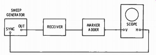
Fig. 4-10. A marker adder is a combination mixer and variable or crystal oscillator,
which adds a marker signal between the receiver and scope. It does not distort
the trace.
Some sweep generators have built-in marker generators, a second variable-signal generator, or a crystal-controlled oscillator. These are superimposed on the sweep frequency and show up as "pips" on the scope trace and identify the frequency at any spot along the trace.
A variable marker can be made to move along the trace, while a crystal oscillator makes several pips along the trace. Also used instead of a variable oscillator is a built-in absorption circuit. The absorption type tends to "suck-out" some of the output frequency, and so shows up as a dip on the scope trace. The absorption type is actually easier to work with since it does not distort the trace, as oscillators some times tend to do. The best method for showing frequency marks on the trace is with a marker adder. This is usually a separate instrument, into which the output of the receiver is fed, and which in turn feeds the scope. It is a mixing and amplifying instrument. Since the marker-generator output does not go through the receiver, it cannot affect the gain, and result in trace distortion (Fig. 4-10).
READING THE SCOPE
The T-axis response being voltage means that the 6-dB down point is at half scale, or a two-to-one voltage ratio between peak E. response and the 6-dB point (dB = 20 log = E2/E1, or 20 log 2, or 6). Thus, with markers you can measure the bandwidth at 6 dB down.
Since the vertical amplifier responds linearly to voltage, it is next to impossible to measure the bandwidth at higher attenuation such as 50 dB down.
THE SWEEP HOOKUP
Connect the sweep generator and scope in the same way as described for a signal generator and VTVM, with one exception. A VTVM has an isolation resistor in its probe to prevent the capacitance of the cable from affecting response at the detector-diode load resistor; a scope has not. Therefore, it is necessary to add a resistor in series with the hot lead of the scope input cable. A 50K resistor is about right. In the case of a product detector, again, a demodulator must be connected to the i-f output, followed by the 50K resistor, and the scope lead (Fig. 4-11).
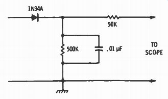
Fig. 4-11. Demodulator and isolating resistor circuit, for use between the
ssb receiver i-f output and a scope.
After the hookup described, the sweep generator should be turned on for about 20 or 30 minutes to stabilize its frequency, or the pat tern will drift across the scope screen. After warmup, turn on the receiver and scope. Set the scope horizontal-amplifier sweep-selector control to LINE, or 60-Hz sweep. This will match the usual 60-Hz sweep rate of the sweep generator. Adjust the focus and intensity for a horizontal line on the CRT. Turn the sweep generator sweep width control to zero. With no sweep the generator acts like a standard signal generator, but is not amplitude modulated. Set the band switch and tuning dial on the sweep generator for the input i-f of the receiver. Rock the tuning control until a deflection is seen on the scope trace. Since the sweep generator is not modulated, there should be no pattern on the scope when on frequency, but rocking the tuning dial develops a low-frequency audio voltage in the output which causes the horizontal line on the scope to move up and down.
Now, turn the sweep control up a little at a time. A hump should appear on the horizontal line of the scope. This is the selectivity curve. The curve may appear right side up or upside down, depending on the phase, which in turn is dependent on the number of amplifying stages involved. It is not important which way the curve appears. An inverted curve can be righted by reversing the connections to the vertical-deflection plates on the CRT, but it usually is not worth the trouble. The sweep-width adjustment should be just enough to show some horizontal line at each end of the curve. The object is to achieve a fully visible trace of the selectivity curve, not too crowded and not overly wide, but just enough to see all parts of the line, its shape and width, as well as height.
Center the trace curve by making slight adjustments to the frequency dial on the sweep generator. If it tends to distort the pattern, make the adjustment simultaneously with adjustment of the phase control on either the sweep generator or the scope. The object is to obtain a centered pattern with straight lines out from each end of the curve.
The output of the sweep generator should be the minimum amount that will provide a clean pattern on the scope without a lot of "fuzz" (noise). Remember that the receiver is to be operated with its sensitivity control wide open. Overloading the receiver with too great a signal will distort the pattern.
Some sweep generators do not go low enough in frequency to work directly into the low i-f stages of a communications receiver. Most low-priced sweep generators are designed for use with TV sets, with i-f's in the megahertz range. In that case, feed the sweep generator into the antenna input with the receiver tuned to one of the lowest amateur bands. In this method, the high-frequency mixer oscillator must not be killed, of course. Connection between the output cable and the antenna terminals must be as close as possible using a minimum of unshielded wire on the hot lead to avoid external signal pickup.
Some sweep generators have a blanking circuit which eliminates the return trace on the scope, and only one pattern appears on the CRT. On sweep generators without the blanking circuit, there will be a curve when the trace moves from left to right and another when the trace moves from right to left. Tuning the sweep-generator frequency-control dial makes the two patterns move in opposite directions. In this case, try to get the patterns together so that they overlay each other. Since sweep generators are primarily designed for TV-set adjustment their maximum sweep width is quite wide. This will re quire a very careful adjustment of the width control, with the control barely cracked open for the very narrow bandwidth of a ham receiver.
Adjust the scope centering controls (height and width) to fill about 3/4 of the CRT face.
ADDING MARKERS
If the sweep generator has a built-in variable marker oscillator, set its frequency to that of the sweep-generator frequency, and turn up its output control a little at a time, until a pip is seen at or near the top of the curve (bottom if the curve is inverted). The pip size should be just large enough to be seen. If the pip is too large, the curve will be distorted. Move the marker tuning dial back and forth and see the pip move off its spot, down one side of the selectivity slope or down the other side, depending on the position of the tuning dial.
The pip size will vary depending on where it is on the curve, since it is affected by lack of gain in the receiver the farther off center frequency you go. To maintain a size that can be seen, you will need to readjust the marker output control as you change frequency. This is not necessary with marker adders.
A built-in crystal oscillator marker will produce harmonics of the crystal and show several markers along the curve. A 100-kHz crystal will produce marker pips every 100 kHz along the curve. This may be fine for TV i-f curves but is too far apart for communication receivers. Crystal oscillators are good for finding the center frequency with crystal accuracy. By plugging in a 455-kHz crystal a pip will appear at the 455-kHz point on the selectivity curve. Five-MHz crystals are common and may be used for 5-MHz i-f's in many ssb transceivers.
Any external signal generator or source of r-f energy may be coupled into the i-f strip of the receiver to show up as pips. Coupling is easy-merely lay the hot lead of the output cable of the external signal generator near the i-f section, or connect it in parallel with the output of the sweep generator to the input of the i-f section of the receiver. A 100-kHz crystal oscillator with 10-kHz and 1-kHz outputs is excellent for putting pips on the trace close enough to measure by. A grid-dip oscillator can also be used, but its accuracy is far from good enough for anything but rough approximations as to frequency.
As mentioned before, the marker adder instrument is ideal for showing marker pips, since the marker-generator output does not go through the receiver.
On a variable marker generator, turn the dial to slide the pip down one slope of the curve until the pip appears halfway between the peak and the base line. Note the frequency. Slide the pip up the slope and over to the other side and half-way down. Note the frequency on the marker-generator dial. The difference between the two frequencies is the bandwidth of the receiver at the 6-dB points.
MEASURING IMAGE RESPONSE
An r-f signal beats with the high-frequency oscillator to change the signal frequency to the intermediate frequency for further amplification. The local high-frequency oscillator may be below the signal in frequency, or above the signal frequency by the amount of the intermediate frequency. If the oscillator frequency is above the signal frequency, as is usually the case at the lower amateur-band frequencies. it would oscillate, for example, at 3.955 MHz to convert a 3.5-MHz signal to 455 kHz. Another signal at 4.410 MHz would also beat with the 3.955-MHz oscillator and produce an i-f signal of 455 kHz. If front end (r-f) selectivity were poor and the 4,410-MHz signal were strong, it would also be heard when the receiver is tuned to 3.5 MHz and interfere with a 3.5-MHz signal. The image is twice the intermediate frequency away from the desired frequency--twice the intermediate frequency above the signal if the oscillator frequency is above the desired signal frequency, or twice the intermediate frequency below the signal frequency if the oscillator is below the desired signal frequency.
With a 455-kHz intermediate frequency, a strong image from one end of the 10-meter band can interfere with the reception of a signal at the other end. Most interference is from other than amateur signals, and they can be strong enough to be quite bothersome. The answer to reduced image interference is improved front-end selectivity or a higher intermediate frequency. Most good ham receivers or transceivers use an intermediate frequency much higher than 455 kHz, especially if they use a dual-conversion circuit. Better amateur equipment i-f frequencies are dictated by the mechanical or crystal i-f filters used in ssb equipment. A common mechanical-filter frequency is 2.1 MHz. Crystal filters also are often in the vicinity of 5.0 MHz.
They may center on 5174.5 or 5501.5 MHz, for example. An image frequency signal at twice one of these higher frequencies hardly has a chance to get through almost any front end.
The setup for making an image-ratio test is similar to the setup for a sensitivity test described earlier. Connect a signal generator with a calibrated step attenuator to the input of the receiver, and turn on the internal modulator. Tune the signal generator and the receiver to the same frequency, around 3.5 MHz. Adjust the signal generator for a low output that will not overload the receiver-something like 50 uV should be good. Note the reading of the VOM or VTVM connected to the output, and note the signal-generator attenuator setting. With the receiver untouched, tune the signal generator to a frequency twice the intermediate frequency above 3.5 MHz, or about 4.410 Mhz if the intermediate frequency is 455 kHz. Turn up the attenuator for more output until a signal is heard. Rock the tuning on the signal generator for on-the-head tuning of the image. Adjust the attenuator until the output meter shows the same output as originally obtained on the first signal frequency. The difference in the two readings from the attenuator, in dB, is the image-response ratio.
If the attenuator is marked in voltage ratio, you will need to convert to dB with the formula: dB = 20 log lower If. for example, the image voltage is 600 times greater than the original signal voltage to produce the same output, the dB attenuation is: 20 log 600 = about 55.5 dB. In other words the image is 55 dB below the signal. It is sometimes called image-rejection ratio, image response, image ratio and signal-to-image ratio.
NOISE FIGURE The limit of the ability to copy a signal is noise. Noise may be external, atmospheric, or manmade; or it may be internal, the result of thermal agitation in components, shot effect in tubes, etc. We noted the sensitivity of a receiver is the signal required to overcome internal noise by 10 dB. The next logical question is, just how much noise does my receiver develop? The answer is the dB of noise developed in the receiver over a perfect noiseless receiver. Receiver noise is designated as N or NF, either of which stands for noise factor or noise figure.
In a good ham receiver, noise developed in the converter stage is overridden by signal amplification in the preamplifier stages ahead of it. In fact the signal affecting receiver noise comes down to the first r-f stage of the receiver. The amount of noise developed is related to the temperature of resistive components in the input circuit, input impedance reflected from the antenna circuit, and impedance of the first tuned circuit. The higher the frequency is, the greater is the noise developed. From a practical standpoint, internal noise becomes important in the r-f stages only above about 25 MHz. Most noise is developed in the mixer stages.
To measure NF of a receiver one needs a source of noise, the output of which is known, or is measurable. The circuit of Fig. 4-12 is a noise generator using a 5722 vacuum-tube diode. It is one you can build yourself and should give you a little better than 20-percent accuracy in making receiver noise measurements. Any accuracy better than that requires a calibrated laboratory-type noise generator.
The 50-ohm resistor in the diode load circuit represents the equivalent of the antenna feeder. For minimum receiver-developed noise, the input impedance of the receiver should match the antenna feeder.
Should it not, by measurement described later, you can get a lower
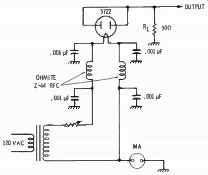
Fig. 4-12. Schematic of a noise generator using a 5722 vacuum-tube diode.
Adjust the heater current to provide a 3-dB increase in noise in the receiver.
The noise figure is 20 I R_L, where I is the current through the diode, and
R_L is the load resistor--in this case 50 ohms.
NF by changing this resistor (RL) to a value equal to the receiver input impedance. However, you would enjoy an actual decrease in noise level only if the antenna impedance were equal to the receiver input impedance.
The noise generator should be built into a metal case with co axial cable output connectors to provide a thoroughly shielded connection to the receiver.
Connect a VOM or VTVM to the output of the receiver. Set its function to read dB or AC output. The receiver must be operated wide open and with the avc disabled by jumping it with a fixed voltage source equal to the no-signal bias developed. An excellent and temporary bias voltage source is a series of flashlight cells. The bfo must be off. although the carrier-reinsertion oscillator must be on for a ssb receiver using a product detector. Connect the noise generator to the antenna input, with close coupling. It is important that no external noise, manmade or atmospheric, enter the receiver.
With the noise generator off and the receiver wide open, read the receiver noise output on the output meter. Turn on the noise genera tor and turn the filament current up until the output meter reads an increase of 6dB or twice the receiver noise alone. When the output is doubled it means the input noise from the generator is equal to the internal noise. Generator noise for this circuit is: 20 IR where, I is the current through the diode circuit.
R is the diode load resistor.
When a 50-ohm resistor is used, as shown in the diagram, NF be comes a direct reading of current in mA. The lower the current is, the lower the external noise is, and. of course, the lower is the internal noise that equals the external noise.
This is a noise ratio that now must be converted to dB by the formula dB = 20 X log current ratio. If, for example, the current is 5 mA. the dB figure for NF is 20 X log 5, or 20 X 0.7 = 14 dB. A good communications receiver runs about 5 to 50 dB for NF at frequencies below about 25 MHz. From a practical standpoint these figures are good for reception of signals through the 15-meter band.
At higher frequencies lower noise figures become increasingly important, but the actual receiver noise figures must be expected to increase at the higher frequencies.
Current through a silicon diode will also produce random noise. A noise generator using a silicon diode in a simple circuit is described later in this section. It is not useful in measuring noise figure of a receiver because the output is not measurable, but it makes a good noise source for aligning receiver front ends.
INPUT IMPEDANCE
In receiving, the antenna is the signal source, with a feed line connecting the antenna to the receiver. Consider the antenna and feeder, then, as a generator and the receiver input as the load. When the impedance of the load is equal to the generator impedance, maximum energy transfer takes place, with the least amount of input circuit noise developed.
Receiver input impedance is a design factor based on the ratio of primary winding to secondary tuned circuit in the antenna coil. Designers do the best they can to make the match perfect, but must compromise for different bands and different frequencies within a band. Sometimes a compromise is made to accommodate the use of random-length antennas instead of a 50-ohm coaxial fed transmitting antenna, or for use with transmission lines of other impedance values.
Section 7 describes an impedance bridge of simple design and easy construction. It requires a source of r-f energy, and a null indicator.
The r-f source can be a grid-dip oscillator, a regular signal generator, or the reduced output of a transmitter driver. The indicator is a high ohms-per-volt VOM, or VTVM. The device acts as an AC bridge with the GDO or other source of r-f as input, and the input of the receiver as the unknown arm of the bridge. When the resistance of the potentiometer equals the unknown impedance, the bridge is in balance and an indicator (VOM or VTVM) will show zero voltage when the unknown is a pure resistance. When the receiver is tuned to the same frequency as the signal source, the receiver input is nearly a pure resistance, but not quite. There will nearly always be some reactance, and this reactance will prevent an absolute null and cause some inaccuracy in the impedance reading. But we are checking for approximate input impedance, so for purposes of seeing how far off the input impedance is from the source impedance (such as a 50 ohm coaxial feed line) the error is unimportant.
Solder a single-turn piece of wire between the inner terminal and the shell of a coaxial connector. Couple the loop to a coil of the GDO for signal pickup. Connect the output of the bridge to the receiver input with coaxial cable. Connect a VTVM to the indicator terminals, with the function switch set to read DC and the range switch on the lowest range.
Adjust the panel control on the impedance bridge for a minimum reading on the meter. Tune the receiver for other frequencies and other bands, and readjust the bridge for minimum each time. The resistance of the control will be the approximate input impedance of the receiver. The value may vary considerably from band to band, and even from one end of a band to the other.
RECEIVER ALIGNMENT
Aligning a receiver means setting the calibration of the tuning dial to read correct frequency as near as possible, adjusting for peak sensitivity, setting i-f tuned circuits for optimum (not necessarily sharpest) selectivity, and setting the bfo or carrier-insertion oscillator for proper sideband operation in an ssb receiver.
Alignment varies from a touchup to peak the performance of a receiver to a first-time alignment of a receiver just built. The amount of work involved varies between the two extremes, and also depends on the type of receiver, whether a single-conversion, dual conversion. a-m, or ssb. In addition there are the filters used in many receivers. There are the sharp crystal filters, and the square top steep-skirt filters, whether crystal or mechanical.
Three things are needed to align a receiver: a source of steady rf (preferably amplitude modulated), a means of reading the output, and the proper-fitting alignment tools. The best input signal device is a signal generator with a good step attenuator in the output. It should have amplitude modulation built-in, as most do. Other acceptable signal sources include the 100-KHz crystal oscillator, either external or built into the receiver. The vfo of your transmitter, if you keep the signal output down (even if it requires a dead short circuit across the output), makes an excellent r-f source. The grid-dip oscillator is an acceptable r-f source for a rough alignment.
A noise generator is good if the receiver is not far out of alignment to start with.
Output indicating devices are simple and can take many forms.
Even the ear can be used by listening to the increase of sound level in the speaker, or the hiss from an unmodulated r-f source, but the ear is not as reliable as a meter indicator. The S-meter on the receiver is a good indicator for an unmodulated r-f signal source.
A VTVM connected across the avc or age bias bus serves in the same way if the receiver has no S-meter. The most frequently used output indicator is a VOM or VTVM across the audio output of the receiver. If the VOM or VTVM has a very low range AC scale, it can be connected across the speaker voice-coil leads, or across a resistor whose value is about equal to the speaker impedance and which is wired in temporarily in place of the speaker. If more voltage is needed, connect the VOM or VTVM across the primary of the output transformer.
A VTVM connected across the second-detector diode load resistor is the best position and type of output indicator, but with avc action replaced with fixed bias. For product detectors a demodulator probe must precede the VTVM. A suitable circuit was described earlier.
With a demodulator preceding it, the VTVM is used on a low-range DC function.
Alignment tools to fit the i-f and r-f trimmers are needed. Where screws are used, as in compression trimmer capacitors, an insulated screwdriver is required. One of the best consists of a tiny metal blade set in a plastic shaft. An all-plastic screwdriver is fine but the end can break off on a hard-to-turn screw. Slug-tuned cores in r-f coils and i-f cans may have a hex-shaped hole or a slot, each requiring a special insulated tool to fit. If a metal screwdriver is used on them, the metal will affect the inductance, and the hardness of the metal could chip out some of the powdered-iron core, even ruining it for use with the proper tool. A hex-ended tool with a narrower neck is handy for adjusting both end cores in an i-f transformer from one end, the hex part fitting all the way through the top core into the bottom for separate adjustment. The tool looks something like Fig. 4-13, Fig. 4-13. A combination insulated alignment tool for i-f transformers. The narrow neck at the right allows the hex end to protrude through the top slug into the bottom.
Both primary and secondary core slugs can be adjusted from one end of the i-f can.
All tuned circuits on a home-brew receiver should be brought into close frequency range with a grid-dip oscillator. With the receiver off, couple the GDO to each of the front end r-f and oscillator coils and adjust them to frequency by setting parallel trimmer capacitors for the high end of each band and adjusting the core slugs (or series padder capacitors if used) for the low end of each band. Intermediate frequency transformers are supplied close enough to frequency so that a rough setting with a GDO is usually not necessary. A check can be made on whether or not they are far off frequency by coupling the coil of the GDO to the coil in the i-f can through the open end of the can. Be sure to use the proper GDO coil, and tune it to the intermediate frequency.
For peaking a receiver for highest sensitivity, the signal source need not be accurately calibrated, but it must be a stable source and capable of fine frequency adjustment, particularly where crystal i-f filters are used in the receiver. For accurately calibrating the receiver tuning dial, the signal source must be close to frequency; a 100-kHz crystal calibrator is excellent for use after rough frequency adjustments are made from some other source.
The receiver should be operated at full r-f gain control setting.
Rest results are obtained if the avc or age bias is replaced with fixed bias, in the manner described earlier in this section for sensitivity measurements. The r-f signal input should be the minimum amount possible and vet show a good indication in the output metering method. It is important not to overload the receiver.
If the receiver is only slightly out of alignment, the signal source may be connected to the antenna input; if it is badly out of alignment. it may be necessary to make a stage-by-stage alignment in the same manner as stage-by-stage gain measurements were made earlier.
In most cases the r-f source is coupled to the converter stage for i-f alignment, and later transferred to the antenna input for r-f adjustments. For purposes of an example, this method will be described in detail.
Lift the shield from the converter tube off the grounding tabs at the socket. The shield will serve as capacitive coupling between the signal generator and the converter tube plate. If the receiver is transistorized. coupling is made to the base of the converter transistor using a .01 uF capacitor between the hot lead of the generator and the base terminal of the converter transistor. Frequently the base input circuit is of such low impedance that the output of the signal generator is insufficient to drive a signal through the converter. In such cases the base connection must be lifted and a 1000-ohm resistor connected from the base to the low end of the coil to which the base was connected. If there already is a resistor from base to ground or to the avc or age bus. and the base is capacitance coupled to the preceding tuned circuits, disconnect the coupling capacitor, and connect the signal generator to the base terminal of the transistor. In most signal generators a terminating resistor (usually about 50 ohms) is in the lead, right at the output end. When connecting directly to the base of a transistor (or the grid or plate of a tube) the DC return path of the terminating resistor can upset bias or plate voltages. If a capacitor is not already part of the circuit under test, add a .01-uF capacitor in series.
AM AND C-W RECEIVERS
If the receiver has a built-in high-selectivity crystal in the r-f circuit, connect a VTVM across the second-detector plate load or diode resistor, and set the VTVM function switch for de. The signal generator should be used unmodulated. The receiver selectivity with crystal in is too great to use a modulated signal because the modulation sidebands would be cut off. If the receiver does not have the crystal, cither the connections mentioned or a VOM or VTVM in the output circuit may be used. If connected to the output, set the meter function switch to read OUTPUT or AC on a low range. The signal generator must then be internally modulated. For either method set the meter for a low range, one that reads the internal receiver noise at about one-third scale.
Set the signal generator to minimum output, and rock the tuning dial around the input intermediate frequency of the receiver. Set the dial at the point of maximum reading on the output meter. The output reading should be about twice that of the receiver internal noise.
Set the signal generator dial carefully for a peak reading on the meter. Now. with the proper alignment tool, adjust each i-f coil for a maximum reading on the output meter. The i-f coils may have trimmer capacitors across each winding. Use an insulated-blade screw driver. and adjust both trimmers, usually located on the top of the i-f can. If the coils are slue-tuned with powdered-iron cores, use the proper tool and adjust both cores. Slotted cores will require adjustment from top on one core, and from the bottom on the other.
Hex cores are usually hollow, and the tool illustrated in Fig. 4-13 will tune both cores from the top. The narrow neck allows you to pass the tool head through the top core down into the bottom core.
Adjust each i-f trimmer or core for highest reading on the output meter. If the signal generator indicates the intermediate frequency is off according to the manual specifications, move the signal generator toward the correct frequency a little at a time, each time re-adjusting the i-f transformers to peak with the signal generator output.
Receivers with crystal-selectivity positions must be adjusted with the crystal in. The crystal establishes the correct intermediate frequency. The procedure is the same as just described except that the signal generator must be much more carefully set since the peaking frequency is very sharp. It is important that the generator has been thoroughly warmed up before making any adjustments, otherwise the slightest drift off frequency will affect your alignment. After alignment with the crystal in its sharpest selectivity position, set the receiver selectivity on a lower position, and. moving the signal generator dial slightly to one side and the other of center frequency, note the output meter readings.
The peak reading should be less than with each side of maximum should be the crystal in, but the drop-off on slower (Fig. 4-14).
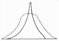
Fig. 4-14. Solid line is selectivity curve with crystal in. Dotted line is
curve in broad selectivity position.
SSB RECEIVERS
Mechanical i-f filters are fixed tuned, and are not adjustable. Crystal lattice filters are also not themselves adjustable, although some have an adjustment to a bifilar winding to make the selectivity top Hatter. These filters establish the intermediate-frequency center. They provide the i-f section with a broad-topped selectivity curve with There are two basic differences between aligning an ssb receiver and the usual a-m type. The ssb receiver does not use a diode second detector (some have both types of detectors and are switchable), and the i-f circuit usually includes a broadband mechanical or crystal lattice filter. To develop DC for the VTVM as an output indicator a demodulator probe or circuit must be connected in front of the VTVM. The input of the demodulator circuit connects to the output of the product detector but with the carrier oscillator killed. The product detector then acts like a simple amplifier. The easiest way to kill the carrier oscillator is to pull the crystal or crystals out of their sockets. If two are used (for upper and lower sidebands), be sure to mark them for return to the proper sockets. The demodulator probe must include an input capacitor to prevent shorting the DC in the plate circuit of the tube or collector circuit of the transistor.
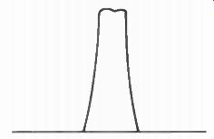
Fig. 4-15. Typical curve of i-f selectivity where a crystal-lattice or mechanical
filter is used.
Mechanical i-f filters are fixed tuned, and are not adjustable. Crystal lattice filters are also not themselves adjustable, although some have an adjustment to a bifilar winding to make the selectivity top Hatter. These filters establish the intermediate-frequency center. They provide the i-f section with a broad-topped selectivity curve with sharp sides. The broad top is usually about 3 kHz wide. The curve looks something like Fig. 4-15. This calls for rather careful adjustment of the i-f transformers to maintain the proper curve. The real selectivity is provided by the filters rather than the i-f transformers.
In many cases the i-f stages do not use dual-winding transformers, but single coils, the purpose of which is to provide the high plate impedance for the i-f tubes for maximum gain.
As an example, the old Swan SW-240 has a four-crystal, crystal lattice filter. Two crystals are cut for a frequency of 5175.5 kHz and two for 5173.5 kHz. The 6-dB down points arc 5176 kHz a 1 d 5173 kHz. for a bandwidth of 3 kHz. The top of the curve has two small humps, reflecting the frequency of the crystals, affected by the bifilar winding. The curve looks like Fig. 4-16. The Swan 500 has a 2700-Hz wide passband in the crystal-lattice filter, the extremes of which are 5500.3 kHz and 5503 kHz.
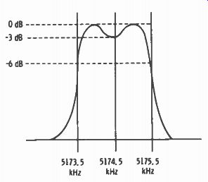
Fig. 4-16. Selectivity curve for the Swan SW 240 transceiver using a crystal-lattice
intermediate-frequency filter.
As you move the signal generator through and to each side of i-f resonance, note carefully the output readings. Look for symmetry in the output on each side of center resonance. The output should be fairly flat for a width of about 3 kHz (check your receiver manual for exact width). There will be slight variations in output between the frequency extremes; but if the variations arc less than 3 dB and are symmetrical, it is considered acceptable. If one side of the flat top is higher than the other, adjustment of the i-f transformers is prescribed. Adjust for equal output of the various humps of the curve.
If there is a bifilar-winding adjustment on the crystal lattice filter, and the humps are more than 3 dB above the dip, adjust the bifilar winding, and re-trim the i-f transformers for equal flat top.
SWEEP GENERATOR
Alignment of the i-f stages is much easier when a sweep generator and oscilloscope are used. You can "see'' what you are doing much easier. The scope will display either the peak reading of a selective a-m receiver or the flat-topped response of an ssb receiver. The great value in using the sweep method is the ease with which symmetry is achieved. Adjustments are made while observing the scope pattern, and every movement made with the alignment tool will be seen as a change in the response on the scope trace.
BFO ADJUSTMENT
On an a-m/c-w receiver, where the bfo does not have a front-panel frequency control, bfo adjustment is made from any steady r-f signal source, even a station carrier. Tune in the signal from the signal generator or other source. The output indicator will be your own ear.
Adjust the bfo trimmer for a pleasant tone either side of zero beat.
Do not adjust the bfo for zero beat. The higher the audio frequency tone you adjust for. the greater will be the attenuation of the signal on the other side of zero beat when you tune your receiver on c-w signals. But the tone must be pleasant and should not tire you while copying code for long periods.
SSB CARRIER-INSERTION ADJUSTMENT
The reinserted-carrier oscillator for the product detector of an ssb receiver is somewhat similar to the bfo in a cw receiver, but with greater stability a requirement. For that reason most good ssb receivers or transceivers use crystal-controlled carrier oscillators, often with two crystals for switchable sideband selection. The crystals are ground to provide a carrier-reinsertion frequency about 300 Hz below the lower limit of the mechanical or crystal-lattice filter for upper sideband reception, or 300 Hz above the upper limit of the filters for lower-sideband reception. The carrier oscillator crystals have trimmer capacitors across them to adjust them exactly right.
The carrier-reinsertion oscillator beats with the ssb signal in the product detector and produces the audio frequencies of the voice.
The frequency of the carrier oscillator must be such as to result in an audio passband between 300 and 3000 Hz. approximately. If the receiver i-f bandpass is 3 kHz wide at the 6-dB down points, that would put 300 Hz down 6 dB at one end, and 3.3 kHz down 6 dB at the other end of the passband. The carrier frequency would then fall farther down on the selectivity curve.
Where the frequency is adjustable it may be done aurally, or by use of a signal generator with built-in variable audio-frequency modulator, or with an audio generator in the transmit mode if it is a transceiver. This last method will be mentioned in the section on transmitter measurements.
Aurally, adjustment is made by first tuning in a good ssb station.
Remove the carrier-reinsertion crystal, and tune the station for highest S-meter reading. Reinsert the crystal and adjust the trimmer across it for best sound quality with proper balance between lows and highs in the speech frequency. If the carrier frequency is set too low on the curve the lower voice frequencies will be lost and the sound will be raspy. If set too high, some of the higher frequencies of the voice will be lost with some loss of intelligibility. In addition when the carrier is set high on the filter response curve, attenuation of the other sideband will be less.
Using a signal generator with built-in variable audio-frequency modulator, connect the generator as described before for i-f alignment. Connect a VOM or VTVM to the output with the meter function switch on OUTPUT or AC VOLTS. Modulate the signal generator at 1000 Hz, and tune the receiver for maximum output meter reading. Turn the internal modulator of the signal generator to 300 Hz; then carefully adjust the trimmer across the carrier oscillator crystal until the 300-Hz signal is 6 dB below the 1000-Hz signal on the output meter.
RECEIVER CALIBRATION
Tuning-dial frequency accuracy depends on proper adjustment of the high-frequency oscillator. Even when correctly adjusted, only the finest receiver will be accurately calibrated clear across each amateur band. The object, then, is to obtain the best compromise of dial markings versus frequency across the band. Making accurate frequency adjustments about Va or Vs of the way in from each end of the band will make the ends and the center of the band fall quite close to exact calibration.
Calibrator adjustments are only as good as the accuracy of the signal source used. If a signal generator is used, it must be a very good one, or one with a built-in crystal-controlled secondary standard which is used to beat against the variable oscillator to set the dial calibration on the head. An excellent source for calibration purposes is the 100-kHz crystal oscillator. Of course, a 100-kHz crystal calibrator limits the dial settings to even 100-kHz points, but this is better than using a less-than-accurate signal generator.
The spread, or tuning coverage, of each band is controlled by proper adjustment of both the capacitance and inductance of each high-frequency oscillator tuned circuit. The high end of the band is set by the capacitance across the coil, and the low end by the inductance of the coil. Low-capacitance trimmer capacitors are across the coil, and are used to fix the high-end limit of the frequency range of the parallel main-tuning capacitor. The high-frequency trimmers are usually screwdriver-adjusted compression types, or screwdriver adjusted cylindrical chassis-mounted types. For the low end. high capacitance compression capacitors are connected in series with the coil and main tuning capacitor, or adjustable coil cores inside the coils are used to adjust inductance. Both types of capacitors arc screwdriver adjusted. The series capacitors are called series padders, and they set the lower limit of frequency effect of the main tuning capacitor. The adjustable powdered-iron cores determine the inductance of the coil.
Connect the signal source to the antenna input. The connection may be made directly to the antenna terminals, or the output cable may be laid near the antenna input. It is only necessary to get a signal into the receiver. Almost any type of output indicator may be used. The S-meter on the receiver is fine. A VTVM across the second-detector diode load resistor, or through a demodulator circuit if the receiver has only a product detector, is OK for unmodulated signal sources. If a modulated signal generator is used, a VOM or VTVM at the audio output is OK. Allow the receiver and signal generator to warm up for about half an hour.
Start with the 80-meter band and set the receiver tuning dial exactly on 3.9 MHz. Set the signal generator exactly on 3.9 MHz.
Adjust the parallel trimmer capacitor for maximum reading on the output meter. Set the receiver tuning dial and signal generator on exactly 3.6 MHz and adjust the series padder or coil core for peak meter reading. This will upset the adjustment made at the high end of the band, so go back to 3.9 MHz and adjust the trimmer again.
Again, this adjustment will change the low-end adjustment, so return to 3.6 MHz and retime. You will find each adjustment affects the other and requires that you repeat each until there is no effect on accuracy. Each time you go from one end to the other the adjustment change becomes smaller and smaller until there is accurate dial readings at both ends. The middle and far ends of the bands should now read accurately also. If they do not. it may require a mechanical shift of the dial or bending the plates of the main tuning capacitor.
These changes affect all bands, however, and are not recommended unless analysis indicates a common error on all bands.
A handy device for knowing which way in frequency an r-f circuit is off is a "tuning wand," which is a long plastic tool with a short piece of copper at one end, and a short piece of powdered-iron slug at the other. Inserting the iron slug into a coil increases its inductance and decreases frequency. Inserting the copper slug into a coil decreases inductance and increases frequency. When doing front-end alignment you can tell which way to turn a trimmer or slug by using the tuning wand to determine if the resonant circuit is above or below the desired frequency.
In those few cases where the front-end resonant circuits have neither an adjustable slug in the coil nor a series padder capacitor, it may be possible to squeeze or expand the coils if they are air wound and self-supported.
Move on to the next-higher band. 40 meters. Use 7.1 and 7.2 MHz for alignment points if your signal source is a 100-kHz crystal calibrator. With a signal generator, use 7.075 and 7.225 MHz for calibration points. Then continue on to the higher bands, picking the nearest 100 kHz point about 14 or 16 in from the band ends.
Some ssb transceivers cover only the phone portions of the bands.
For these, select the nearest 100-kHz points in from the ends, or at the band ends marked.
If a 100-kHz crystal calibrator is used as a signal source it should itself be calibrated against WWV. All crystal calibrators have a trimmer capacitor across the crystal which allows you to zero beat the crystal against the WWV signal standards. If your receiver is a ham band only receiver, you will need to enlist another general-coverage receiver somewhere. WWV broadcasts from Ft. Collins, Colorado are on 2.5, 5, 10, 15, 20, and 25 MHz. Also. WWVH in Hawaii is on 5, 10, and 15 MHz. The signals provide pure cw, 400- and 600-Hz tones, time, and propagation information. Zero-beat the 100-kHz crystal during the pure unmodulated signal periods.
Using the 100-kHz crystal calibrator on the higher amateur bands requires care to select the right 100-kHz harmonic. Use a signal generator or other reasonably accurate signal source to find any even 1-MHz point, and pick up the 100-kHz crystal calibrator signal near it. From there you can find the proper 100-kHz points inside the edges of the bands by counting the beat notes up or down from the 1-MHz point. In the vhf bands, finding the right 100-kHz point is very difficult, and may be impossible. The 4-MHz bandwidth of the 6-and 2-meter bands contain 41 100-kHz points from one end to the other. For the vhf bands the 1-MHz points from a decent signal generator usually give sufficiently accurate calibration points, except for the very particular ham.
If we seem to have overlooked the popular grid-dip oscillator for alignment, it is only because its accuracy is not nearly good enough for calibration, and too often its signal is not stable enough for front end peaking. Battery-operated GDO's have better stability since they are independent of the AC line, and could be used for peaking, lacking a better signal source.
FRONT-END ALIGNMENT
It is the alignment of the preamplifier stages that provides the best usable sensitivity. Peaking the front end will not provide a great deal of overall again improvement, but peaking does provide the improved signal-to-noise factor. The more you can bring the signals up over the internal receiver noise the better the receiver performance will be.
The setup with a signal source is similar to the one for calibration but without the need for calibration accuracy. The same kind of adjustments arc made to the antenna and r-f coils, and in the same manner, as for the oscillator circuits. Keep going back and forth between the two ends of the bands and adjust parallel trimmers and series padders or coil cores for highest reading on the output meter.
One of the best signal sources for improving signal-to-noise ratio is a noise generator. Where we just want an improvement, but not measurement, a simple solid-state diode circuit for a noise generator is good enough, instead of the vacuum-tube noise generator described ...
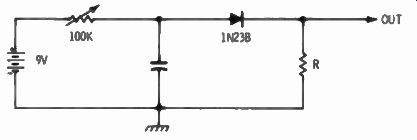
Fig. 4-17. An uncalibrated but adequate
noise generator for peaking the receiver front end.
...earlier in this section. Fig. 4-17 is the circuit diagram of a simple noise generator anyone can build. The variable resistor varies the current through the diode and the output of the noise generator.
USING THE NOISE GENERATOR
The noise generator must be well shielded, and should be connected to the receiver antenna terminals as close as possible. It is important that a minimum of outside noise pickup get through. Turn the receiver gain controls wide open, and get a noise reading on the output meter with the noise generator off. You will be reading the receiver noise. Turn on the noise generator and adjust the variable control until you read about twice the noise that you did from the receiver alone. Adjust the antenna and r-f stages at about 1/4 or 1/3 in from each end of each band for an increase in output of noise.
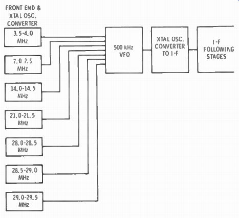
Fig. 4-18. Very tine receivers have a single vfo with only 500-kHz range (some
200-kHz) for a high stability and accuracy. Front-end sections are each 500-kHz
wide, and have separate crystal-controlled converters to make use of the single
vfo.
Reduce the noise-generator output with each increase in output-meter reading as you make the peaking adjustments. Go back and forth between the two ends of the bands, on each band, until there is no increase in noise signal with adjustments.
HIGH-PRICED RECEIVERS
The very best receivers have multiple-conversion circuits, with segmented or multiple-band front ends. A common 500-kHz wide vfo is used on all bands, and provides high stability and accuracy. It may feed directly into the IF stages, or be followed by a higher-frequency, crystal-controlled conversion stage before the i-f stages. The vfo is preceded by separate 500-kHz wide front-end sections (Fig.4-18), each with its own crystal-controlled conversion stage to convert for use with the common 500-kHz vfo. There are variations of the one sketched here. Some receivers locate the vfo in another part of the circuit. At least one receiver has 200-kHz segments.
Calibration is simplified, in that there is only one variable-frequency oscillator to calibrate. The other conversion mixers being crystal-controlled need no calibration adjustments. Front-end peaking is the same as described before, except there will be more bands to peak (there are three segments to the 10-meter band) with 500 kHz segments, and still more with 200-kHz segments.
Because of the very high sensitivity and selectivity of these fine receivers, it takes a laboratory type signal generator to do a good job of alignment.