On the basis of frequency of use and low-cost investment, the instruments described in this section should be a part of every ham shack equipment list. Most of these can either be purchased at low cost ready to operate; or they can be built from reliable kits, or from amateur manuals or magazine articles. Information is given in this section on how to build the SWR bridge, impedance bridge, and the coupling and phasing network of a monitoring scope. There are any number of magazine articles on how to build a crystal calibrator, but the one shown here is as inexpensive coming from a ready-to-assemble kit as building from scratch. Grid-dip oscillators are easily home built. also, except for the need to calibrate them for each coil of the set. Kits include the calibration and may be a better bet for the amateur than building from scratch. The transistor checker described in Section 3 is a simple go-no-go type that will tell if a transistor is good or bad, but it will not indicate the gain in numbers. It is a good instrument to have around to check out a drawer full of transistors, or for selecting the best of a package of bargain transistors.
VOM
With the large number of high-sensitivity VOM's being imported, there is no excuse for an amateur not having a VOM in his shack.
These days it is important to use a high-sensitivity VOM. The old standard 1000 ohms-per-volt VOM should be considered out of date.
Transistors operate at a very low voltage, which means that a VOM will be operated on its lowest scale most of the time. A 1000 ohms per-volt VOM will usually be used on its lowest scale. If this is the 5-volt scale, it will look like a 5000-ohm load at all times when making transistor measurements. This could be much too low a load, especially when testing for base voltage.
VOM's of 10,000 ohms/V and 20,000 ohms/V ''look like" resistor loads 10 times and 20 times that of a 1000 ohms/V VOM. A high quality 20,000 ohms/V is a bit expensive, but it should be your first consideration; if you cannot afford one, a lower-cost imported 20,000 ohms/V VOM is better than a high-quality 1000 ohms/V VOM. Another place where a high-sensitivity VOM is important is when one is used as a bridge indicator, as in the antenna impedance bridge described later. A grid-dip oscillator may be used as the signal source if a high-sensitivity VOM is used for a null indicator.
The VOM has the advantage of being portable. This is especially handy when it is necessary to go outdoors and make impedance or resonance checks on an antenna (Fig. 7-1 ).
VTVM
Much higher sensitivity is an advantage of the VTVM over the VOM. It usually has a constant input resistance of at least 11 meg ohms. More and more transistorized VTVM's are coming on the market, and these will provide the portability of a VOM (Fig. 7-2).
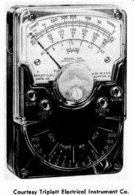
Fig. 7-1. This pocket-sized VOM measures only 2-3/4" x 4-1/4" x
1-5/16". It has 20.000 ohms-per-volt sensitivity. Courtesy Triplett Electrical
Instrument Co.
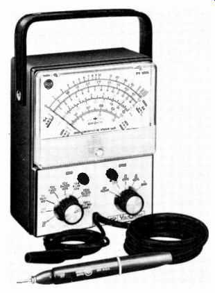
Fig. 7-2. In every respect this instrument is like an AC operated VTVM, but
it is transistorized and battery-operated. Courtesy RCA
However, these are generally higher priced than the AC operated VTVM. which has the high sensitivity so important to checking amateur equipment but depends on an AC source for prime voltage (Fig. 7-3). If cost is a factor, consider building a VTVM from a kit from one of several manufacturers with established reputations.
Since amateur equipment operates at high frequencies, a worth while investment is an r-f probe for the VTVM. With it you can make actual measurements of voltage at high radio frequencies.
SWR METER
The SWR meter may be called by several names: SWR bridge, reflected-power meter. VSWR meter, etc. The instrument reads the ratio of forward power to reflected power going from the transmitter into the feed line, and indicates the mismatch of the antenna to the feedline. SWR means Standing Wave Ratio. When power is reflected back down the feed line due to a mismatch of the antenna to the feed line, standing waves are developed on the feed line. The greater the mismatch is. the greater are the standing waves. A perfect match leaves no standing waves, and is said to have a 1:1 standing-wave ratio.
A low SWR is important only in coaxial-type cable using a solid dielectric between the inner conductor and the outer shield. The di electric introduces losses. Tables on cables show this as so many dB of attenuation per hundred feet of cable, and the higher the frequency is, the higher the attenuation is. The losses shown in the tables apply to the forward current only; that is, when there are no reflected waves, or the SW R is 1:1. A mismatch between the feed line and the antenna will result in a higher than 1:1 ratio, and the standing waves will introduce additional losses, depending on the ratio. The higher the ratio is. the higher the losses will be on the feed line. Sec Section 6 for more information on this and appropriate tables on cable attenuation.
The big advantage of an SWR bridge like those shown here is that it can be left in the line at all times. It can handle the full output power of any transmitter and introduces practically no losses. In this way you have a constant check on output conditions. Figs. 7-4 and 7-5 show two SWR meters available in kit form.
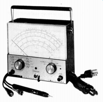
Fig. 7-3. This VTVM features an unusually large meter scale. The DC input
resistance is 16 megohms, as compared to the usual 11. Courtesy Simpson Electric
Co
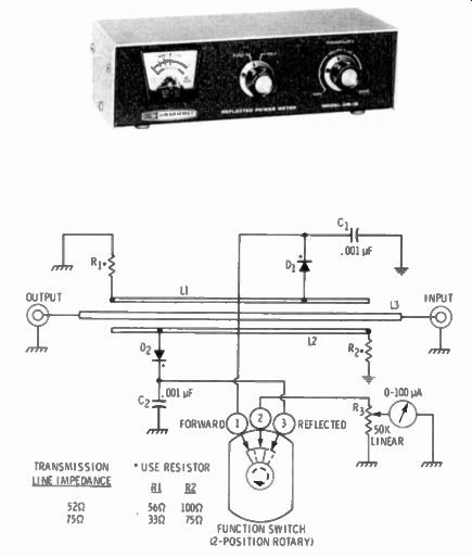
Fig. 7-4. A popular SWR meter in kit form is the Heathkit unit. Both the pickup
section and indicator are in a single case. Courtesy Heath Co.
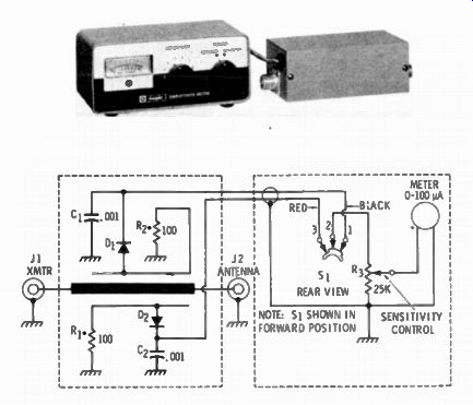
Fig 7-5. The Knight-Kit SWR meter is in two parts. The pickup unit can be
located near the transmitter output and the indicator placed anywhere on the
operating table.
1. CAPACITORS INDICATED IN MICROFARADS.
2. RESISTORS INDICATED IN OHMS.
3. K x 1000 OHMS
• VALUES SHOWN ARE FOR 72 ohm LINE.
• WHEN USING A 52 ohm LINE, VALUES OF R1 AND R2 ARE 160 ohm
Courtesy Allied Radio Corp.
BUILDING THE SWR METER
An SW R meter is easy to build. Construction is mostly mechanical.
The one described here is in two parts, the part connecting in series with the transmission line is separate, so it may be connected with out bringing the transmission line up to the operating table. The indicating meter and switch are a separate unit to be located at the operating position for easy visibility. A 5-inch X 214-inch X 214-inch Minibox contains the transmission-line elements.
Fig. 7-6 is a photograph of the front view of the indicator part and closed Minibox. The meter, switch, and sensitivity control can be mounted in a metal box also. Shown here is a piece of perforated Masonite supported vertically to a wood base. The indicator elements need not be shielded. Fig. 7-7 is the rear view of the indicator section and the open box of the bridge parts. Fig. 7-8 is the schematic diagram.
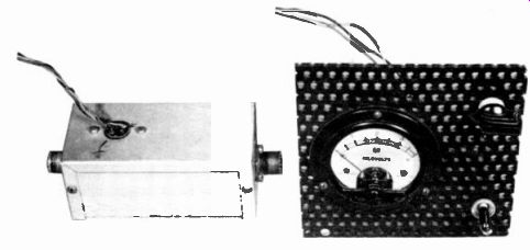
Fig. 7-6. Front view of the home-built SWR meter. The panel meter is mounted
on a Masonite board, but it can be enclosed in a box if preferred.
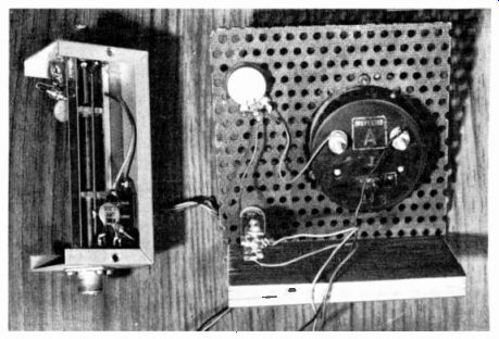
Fig. 7-7. Rear view of the SWR meter with cover removed from pickup section.
Fig. 7-8. The schematic diagram is fairly standard, and this one is similar
to many others. A lower-sensitivity meter may be used, but it will take higher
power at the lower frequencies to read full scale.
-----------------
PARTS LIST
1 1 1 1 2 2 2
100-mA meter movement spdt switch 50,000-ohm potentiometer
5" X 2'4" X 2'4" Minibox 5" X %" metal strips (solder able)
female coax chassis connectors.
IN34A (or any r-f type) matched diodes
2 2 2 2 1 2
150-ohm, 1/4-watt resistors , 0012-uF ceramic capacitors 4-inch pieces # 12 copper wire 3 4-inch square polystyrene blocks 4%-inch piece 1/4-inch copper tubing 2-terminal wiring tie points
-----------------
Mount the female coax chassis connectors one to each end of the U-shaped half of the Minibox (like the one shown in Fig. 7-5). Cut two 1/4-inch squares of polystyrene sheet 1/16-inch thick. Drill 14 inch holes in the centers of the polystyrene squares, and slip them over the copper tubing. The polystyrene blocks will act as spacers for the metal strips and will support the pickup wires. Solder the ends of the copper tubing to the center terminals of the connectors. Place solder lugs under each opposite screw used for mounting the coax connectors, and solder the ends of 5-inch X 1/2-inch metal strips to the solder lugs so the strips face the copper tubing on opposite sides and are spaced 1 á -inch from it. Any kind of metal will do except aluminum, as long as you are able to solder to it.
Cement 4-inch lengths of copper wire to the polystyrene blocks, one on each opposite side of the tubing, using Duco or similar cement. Wire the rest of the components between the copper pickup wires and ground lugs or terminal tie points, as shown in the schematic diagram. Be sure to keep leads as short as possible. This will require using heat sinks on the diode leads as well as on the resistor leads. Be sure the polarities of the diodes are the same. If the SWR meter is to be used with 52-ohm cable, use 150-ohm resistors for pickup-wire terminating resistors, or if it is for 75-ohm lines, use 100-ohm resistors. For greater accuracy use close-tolerance resistors and matched diodes.
Sensitivity depends on the length of pickup unit, sensitivity of the meter movement, and the frequency involved. The components and construction shown here will operate at 80 meters with power inputs of about 75 watts and up. For greater sensitivity use a 50-uA meter movement, or add a transistor amplifier ahead of the meter.
The meter panel shown in the photograph is part of a "junk-box" meter with markings from 1-4. SWR figures can be calculated from any meter markings on the basis of assuming a figure of 10 for the top of the scale, using this formula: SWR = + X 10 - X where, x is the reflected-power reading, for example, if the reflected reading is 2, 10+2 12 SWR = {-h -s = = 1-25 or a ratio of 1:1.25 1 V Z o In use the switch is set Forward and the sensitivity control is adjusted for full-scale indication of 10. The switch is then flipped to Reflected and the meter is read, and the reading applied to the above formula.
The forward position may be used to determine relative power output for transmitter tuning. Since power output varies as the square of output current or voltage, make up a table of relative power versus the meter figures. With a full scale of 10 the table will look like this:
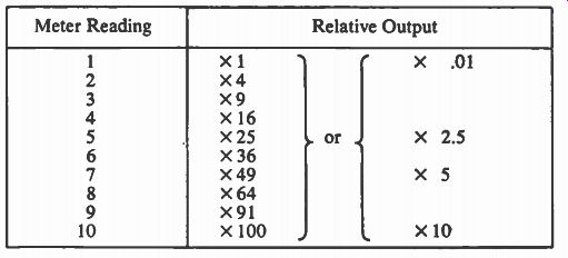
-------------- Meter Reading , Relative Output
You can make your own overlay scale for the meter with two ranges, one for Forward relative power and the other for Reflected, but in terms of SWR. The SWR scale will be about like this:
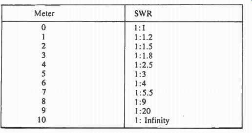
------------------ Meter SWR
ACCURACY
Several factors affect the accuracy of a home-built instrument such as this. Stray component capacities and inductances of their leads will make some higher-frequency readings different than lower frequencies. Diodes are inherently nonlinear at low current. Low power through the SWR meter will have greater inaccuracy than high power.
Harmonics generated by the transmitter will affect the readings.
Twenty-meter harmonics from a 40-meter output will make a 40 meter antenna look highly mismatched. Reflected power from the 20 meter harmonics will show up as a higher-than-correct SWR on the meter.
USING THE SWR METER
The SWR meter (or the pickup part if it is a two-unit instrument) is connected in series with the transmission line between the transmitter and the transmission line. The design of the unit (determined by the pickup lead terminating resistors) must match the characteristic impedance of the transmission line. Turn on the transmitter and resonate it for the frequency you are interested in, matching to the resonant frequency of the antenna. Turn power on and adjust the sensitivity of the SWR meter for full-scale reading with the switch in the Forward position. Without touching anything else, flip the switch to Reflected and read the SWR, using the foregoing table if a scale has not been made.
Regardless of the accuracy of the SWR meter, a high SWR reading means there is a poor match between the feed point of the antenna and the transmission line and/or the antenna is not resonant at the operating frequency. The object is, of course, to trim the antenna to exact resonance, and to match the impedance of the center of the antenna to the characteristic impedance of the line. Each adjustment can be made using the SWR meter. Trim the antenna a little at a time until the SWR meter indicates the lowest ratio. The antenna is then resonant. Then adjust for a match by means of a T- or gamma-matching system (or a proper matching stub) for a ratio of 1:1 on the SWR meter.
IMPEDANCE BRIDGE
A true bridge has four ratio arms. When each pair of resistances are equal the bridge is in balance. Fig. 7-9 shows the basic circuit of the impedance bridge we are about to describe. Two 51-ohm fixed resistors comprise one pair of arms. It is not important that these resistors be exactly 51 ohms but they must be exactly equal to each other.
The other pair of arms consists of a variable resistor and the unknown resistance. When the variable resistor is adjusted to be equal ...
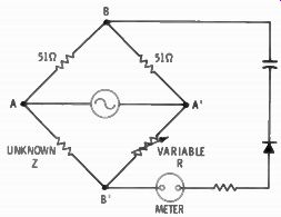
Fig. 7-9. The basic schematic of a bridge. If the variable arm and the unknown
impedance are the same, the bridge is in balance, and the meter will read zero.
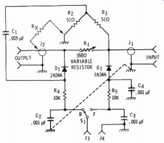
Fig. 7-10. The schematic of the homebuilt impedance bridge. The part of the
circuit below and to the right of the dashed line is for reading r-f input-an
added feature.
... to the unknown resistance, the bridge is in balance, and the value of the unknown impedance is read on the calibrated variable-resistor dial scale. Note the connection of the source of voltage and the indicator in the circuit. When a source of AC r-f voltage is applied to terminals
------------------
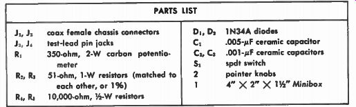
PARTS LIST
J1, J 2 coax female chassis connectors Jj, test-lead pin jacks Ri 350-ohm, 2-W carbon potentiometer R?, Rt 51-ohm, 1-W resistors (matched to each other, or 1 %) R1, Rj 10,000-ohm, 1/4-W resistors D,, D1 1N34A diodes C1 0.005-uF ceramic capacitor C 2 , C3 .001-/xF ceramic capacitors Si spdt switch 2 pointer knobs 1 4" X 2" X Minibox
------------------
A and A', no voltage will develop between terminals B and B', and the meter will read zero if all arms are in balance.
The schematic of the impedance bridge we are describing is shown in Fig. 7-10. It is similar to the basic bridge circuit except for the addition of a means of reading relative input voltage, and switching from input reading to bridge reading. The addition is below and to the right of the dashed line. This part may be omitted, and is in many such circuits. The input reading permits readings for SWR. The primary object of this instrument is to read input impedance to a transmission line or the center of an antenna, however. Fig. 7-11 is a front view, and Fig. 7-12 is a rear view with the cover off.
This impedance bridge will do a fairly accurate job of reading impedance in all amateur bands through the 10-meter band. Above that frequency stray capacitances and lead inductances affect accuracy.
Commercial bridges are available with precision construction for reading impedance at much higher frequencies (Fig. 7-13). None of the parts for the bridge are critical except the two 51-ohm resistors. (RR ) which should both be the same resistance, even if not precisely 51 ohms. All parts fit inside the 4" X 2" X 1(6" Mini box. You could use a larger box and mount a 50-uA meter movement in it. This instrument is designed for use with an external VOM of high sensitivity. This keeps the cost of the bridge down, although one with a built-in meter is handier to use.
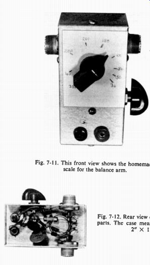
Fig. 7-11. This front view shows the homemade scale for the balance arm.
Fig. 7-12. Rear view of bridge showing parts. The case measures only 4" X 2" X W.
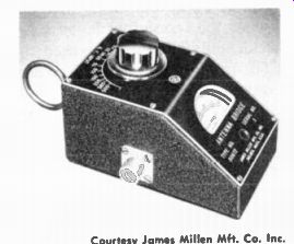
Fig. 7-13. An impedance bridge for use up to 140 MHz. It has a variable capacitor
for a bridge arm instead of a variable resistor. Note the loop on back for
coupling to a GDO for signal source. Courtesy James Millen Mit. Co. Inc.
CONSTRUCTION
Those parts that are part of the bridge circuit must have short leads and be spaced for a minimum of capacitive coupling between them. This involves the bridge resistors, the two diodes, and the .005 capacitor. The rest of the parts are decoupled from rf and may be placed anywhere. If the metal box is painted, be sure to scrape the paint away where grounds are made.
After the instrument is assembled and wired, cut out a white card and place it under the potentiometer mounting nut. Connect an ohm meter to the terminals of the pot and mark off important resistance points on the card as measured on the ohmmeter. A more precise calibration is made with a signal generator connected as a voltage source and a variety of accurate resistors connected to the output coax connector. Set the generator for the highest frequency you expect to use, and balance the bridge for minimum reading on the VOM with each resistor, marking the value on the scale card.
USING THE IMPEDANCE BRIDGE
Unlike the SWR meter this impedance bridge cannot be left in the transmission line, nor used with high power. Any more than four watts of r-f fed into the bridge is likely to burn out the variable resistor arm of the bridge. Users find this is the one component most frequently replaced when the transmitter is used as the signal source and the output is accidentally allowed to exceed the power handling limit of the bridge. The transmitter may be used as a source of signal input provided its output is held down, by a voltage-divider resistor network, limited carrier injection in the case of a ssb transmitter, or by using the exciter only. A better source of rf is a signal generator or a vacuum-tube type grid-dip oscillator, although these require the use of a sensitive VOM or VTVM as a null indicator. Fig. 7-14 shows in block diagram form how a GDO is coupled to the bridge to measure the impedance reflected from the transmission line. Fit a coaxial connector with a 1- or 2-turn link having a diameter just right for going over the GDO coils, and tightly coupled.
Be sure to mark the side of the case as to which side is for the un known (X transmission-line connection), and which is for the source ...
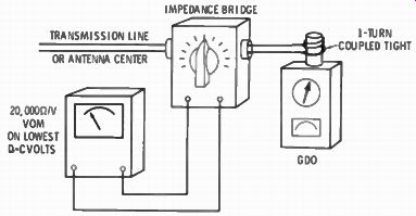
Fig. 7-14. The hookup of an antenna impedance bridge.
... of r-f power. Use adhesive tape and write on it. or punch a tape from a label maker. Refer to the schematic diagram for “In" and "Out." "In" is the signal-source side.
Depending on the sensitivity of the VOM used as the balance indicator, the GDO control may have to be turned all the way up for enough signal power to give a good indication on the meter. When the variable resistor is set at a point where a null in the meter reading is indicated, the bridge is balanced and the unknown impedance can be read from the calibrated dial scale. This measurement is made with the switch in the "R" position.
The bridge may also be used to measure SWR. Furthermore, it may be used for unbalanced lines of any impedance. Set the balance arm for the characteristic impedance of the line, and place the switch on the side for reading input rf ("F" position). Adjust the coupling of the GDO and its control for full scale reading on the VOM. If full scale reading cannot he obtained, use any voltage figure on the VOM scale for a reference, and call it 10. Switch to bridge reading on the side switch (position "R"). read the voltage on the VOM, and convert it to ratio of the reference 10. Refer to the graph of Fig. 6-14. of Section 6, and read SW R 100-kHz
CRYSTAL CALIBRATOR
Inexpensive to buy and easy to build, a 100-kHz crystal oscillator should be permanently connected to every amateur's receiver, if it is not already built in. The one shown in Fig. 7-15 may be attached to ...
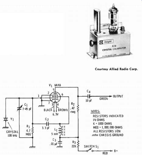
Fig. 7-15. The Knight-Kit 100-kHz crystal calibrator fastens to the back of
a receiver, and takes its power from the receiver. Courtesy Allied Radio Corp.
Fig. 7-16. The schematic diagram of Fig. 7-15. Add a 1N34A diode in series with the output for richer harmonics, reaching well over 30 MHz.
NOTES: RESISTORS INDICATED IN OHMS K • 1000 OHMS MEG • 1.000.000 OHMS ALL RESISTORS 1/2W CHASSIS GROUND
... the back side of a receiver, or mounted inside if there is room. The calibrator receives its power from the receiver power supply. The schematic (Fig. 7-16) is typical of circuits using a vacuum tube.
Design is such that the oscillator is rich in harmonics, and so produces not only a signal at 100 kHz, but harmonics every 100 kHz up to above 30 MHz. The higher the harmonic number is. the weaker is the signal produced. In this particular circuit adding a 1N34A diode to the output between the 10-pF capacitor (marked C.) and the output will increase the strength and limit of harmonics.
Almost any transistor is capable of oscillating at 100 kHz and may be used as an oscillator controlled by a 100-kHz crystal. One of the...
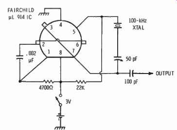
Fig. 7-17. An integrated circuit (IC) 100-kHz crystal calibrator. It operates
from a 3-volt battery.
...latest uses an inexpensive Fairchild /zL914 IC (integrated circuit). The circuit used is shown in Fig. 7-17. The current drain is so small that the calibrator will just about run forever on the 3-volt battery.
The amateur magazines frequently show frequency-divider circuits that may be added to the output of the 100-kHz oscillator to supply markers at 10 kHz and even 1 kHz. These are flip-flop circuits whose constants are such that the 100-kHz oscillator will lock the 10-kHz oscillating circuit into step to produce exact 10-kHz markers, etc.
The quartz crystals are cut in such a way that a small variable capacitor across or in series with the crystal will adjust the crystal frequency to exactly 100 kHz. By using an all-wave receiver and tuning to one of the WWV signals (carrier only) the crystal may be adjusted for zero beat. Thereafter exact 100-kHz markers can be read on the receiver.
GRID-DIP OSCILLATOR
The name itself describes the grid-dip oscillator operation-an oscillator in which the grid current dips when energy is absorbed from its resonant circuit. As with all vacuum-tube oscillator circuits, feedback from plate to grid sustains oscillation. The r-f voltage across the resistor between grid and ground produces a DC current through the resistor as a result of the rectifying action between grid and cathode (Fig. 7-18). A meter in the grid circuit will read the direct...
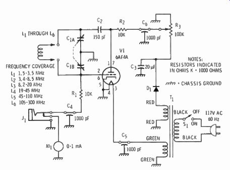
Fig. 7-18. The schematic of the Knight-Kit grid-dip oscillator is typical
of many using a vacuum tube. The Colpitts oscillator circuit permits using
two terminal plug-in coils. Courtesy Allied Radio Corp.
...current. In a free-running oscillator the voltage at the grid is high, and, therefore, the current is high. Power absorbed from the resonant circuit reduces the grid voltage and. thus, the current. When the coil of the resonant circuit is coupled to an external resonant circuit, power is absorbed when the two circuits are mutually resonant. Thus a dip in grid current indicates mutual resonance, and the calibrated dial indicates the frequency of the external circuit.
To increase the utility of this valuable little instrument, the circuit is usually designed to permit other functions. By reducing the plate voltage to zero, oscillation stops and the grid and cathode act as a diode to indicate energy picked up from an external "live" resonant circuit, and so the GDO is used as an absorption wavemeter. By plugging headphones in series with the plate and operating the circuit as an oscillator, you can hear the beat note between its own oscillations and an external signal-thus it can be used as a beat-frequency detector. Of course, as an oscillator, its signal can be picked up in a receiver, and it becomes a signal generator.
Plug-in coils are used to cover a wide range of frequencies, up to as high as 300 MHz. The highest-frequency coil is usually a hairpin or half-turn coil.
SEMICONDUCTOR GDO's
Vacuum-tube GDO's are vigorous oscillators and quite sensitive to the effects of an external resonant circuit. Battery-powered, portable GDO's using semiconductors are handier to use, especially outdoors on an antenna. High-frequency transistors, especially the high-impedance FET type, make excellent oscillators, although they frequent ly require a following amplifier built in to increase their sensitivity and operate a meter.
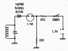
Fig. 7-19. The basic tunnel-diode GDO circuit. Sensitivity is low, and the
meter should be preceded by an amplifier, as shown in Fig. 7-20.
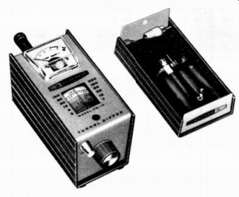
The tunnel diode has negative resistance characteristics and makes an excellent oscillator good for very high frequencies. A fundamental circuit is shown in Fig. 7-19. While this circuit is usable as shown, meter deflection is quite small unless it is coupled tightly to an external resonant circuit. The circuit of Fig. 7-20 is a complete tunnel diode type GDO with a three-stage transistor amplifier to increase its sensitivity for more positive meter action. The photograph of Fig. 7-21 shows the completed unit, which is built from a commercial kit.
MONITORING SCOPE
Because the electron beam in a cathode-ray tube has no inertia, it reacts instantaneously to voltages impressed on its deflection plates.
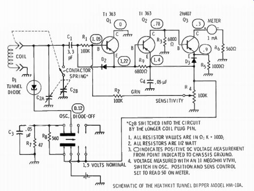
Fig. 7-20. A three-stage transistor amplifier is used to increase sensitivity
in the tunnel-diode GDO. Courtesy Heath Co.
SCHEMATIC OF THE HEATHKIT TUNNEL DIPPER MODEL HM10A. C2B SWITCHED INTO THE CIRCUIT BY THE LONGER COIL PLUG PIN.
1. ALL RESISTOR VALUES ARE IN Q. K x 1000;
2. ALL RESISTORS ARE 1/2 WATT
3. OINDICATES POSITIVE DC VOLTAGE MEASUREMENT FROM POINT INDICATED TO CHASSIS GROUND.
4. VOLTAGE MEASURED WITH AN 11 MEGOHM VTVM. 1.5 VOLTS NOMINAL SWITCH INOSC. POSITION AND SENS CONTROL SET TO READ 50 ON METER.
The best way to "see" what is happening in the output of a transmitter is by means of an oscilloscope, not only for alignment and adjustment, but as a continuous monitor while transmitting.
The method used is to apply the r-f voltage of the transmitter output to the vertical-deflection plates, while audio from the transmitter or the internal sweep of a standard scope is applied to the horizontal plates.
Only expensive laboratory type scopes will handle rf at amateur frequencies through their vertical amplifiers. However, since the output voltage of a transmitter is high, it can be connected directly to the vertical-deflection plates without going through the internal amplifier. Then, an inexpensive general-purpose scope may be used (Fig. 7-22). Some instruments have facilities on the back for making the direct connections to the vertical-deflection plates. Some instruments have only an access opening on the back of the case. Where there is no access, it will be necessary to cut an opening or install binding posts on the back.
The CRT mounting socket is always on the back, and generally very close to the back panel of the case. Access to the terminals on the socket is usually fairly easy. Do not disconnect any of the circuits to the plates, since DC must remain connected if the rest of the focusing and centering circuit is not to be disturbed. Capacitance coupling to the deflection plates through a pair of .01-uF ceramic capacitors is all that is necessary.
Courtesy Heath Co.
Fig. 7-21. A tunnel-diode GDO made from a kit. Plug-in coils cover the range from 3 to 260 MHz.
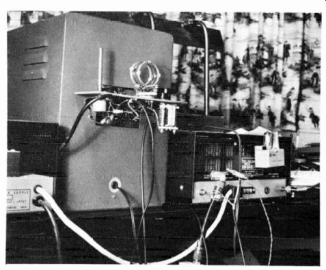
Fig. 7-23 is a photograph of the circuitry added to the back of a general-purpose
scope. All components are mounted on a Masonite shelf. To the right is a tuned
circuit using plug-in coils. The tuned circuit is link-coupled to a pickup
loop which is coupled to the transmitter output tank, or is capacitance-coupled
to the inner conductor of a coaxial transmission line. On the left is an audio
phasing circuit to correct the phase of the audio output from the transmitter
before applying it to the horizontal input of the scope. The circuit is shown
in Fig. 7-24.
A basic scope without amplifiers and a sweep circuit is easy to build, and some are shown in amateur handbooks. These are good only for monitoring an a-m transmitter because of the high voltages needed for the deflection plates. For example, a 3AP1-A CRT commonly used in basic scopes needs peak-to-peak signals of from 50 to 90 volts per inch of deflection. Such voltages are easily available from the modulator and from the r-f output of a-m transmitters; but ssb transmitters will have only very low audio voltages available, ...
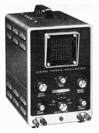
Fig. 7-22. Any inexpensive oscilloscope will serve as a modulation monitor.
This one is available in kit form.
...which will require further amplification for deflecting the horizontal plates of the CRT. Therefore, a general purpose scope with a horizontal amplifier is needed, and these are better purchased (even if in kit form) than built from scratch. A sweep circuit is needed for voice monitoring an ssb transmitter.
Fig. 7-23. A home-built "add-on" for applying transmitter rf to
the vertical plates of a CRT in an oscilloscope. R-f pickoff is from the center
conductor of a cut coaxial connector, shown at the lower right of the photo.
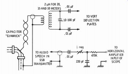
Fig. 7-24. Diagram of the monitoring hookup. A plug-in coil, trimmed to 2
covers 20. 15, and 10 meters with a 100-pF variable capacitor. The audio phasing
network is shown below.
COUPLING RF
Very often rf may be obtained from the coaxial transmission line and coupled directly to the vertical-deflection plates of the CRT. A 200-watt transmitter will develop 100 volts of rf between the center terminal of a 50-ohm line and ground. The peak-to-peak value is about 280 volts, enough to develop a three-inch high pattern on the face of the CRT. Since the voltage to the deflection plates will vary with power and frequency, it is best to provide some means of adjustment, and of increasing the voltage when necessary. The answer is in a tuned circuit as shown in Fig. 7-24. The coil and capacitor values shown will resonate in the 20-, 15-, and 10-meter bands by adjusting the variable capacitor. The coil used was a cut-down plug-in, coil which was quite popular back in the days of plug-in coils for the bandswitching of transmitters. It includes an adjustable link, although it is not necessary. A coil and capacitor of your own design may be used, with currently available air-wound coils. A 2-inch diameter, 21ó-inch long coil with 25 turns will resonate in the 80- and 40 meter bands with a 100-pF variable capacitor. A tap at 5 1/2 turns will have the right inductance to tune the 20-, 15-, and 10-meter bands. Couple a 2-turn link of insulated wire to the bottom of the coil, and use a piece of coaxial cable to the r-f source. When tuned to resonance the voltage available for the deflection plates is quite high. If the pattern goes off screen, merely detune the circuit until the pattern is the desired size.
The lower right portion of the picture of Fig. 7-23 shows a good method of tapping off rf from the transmission line. A slice is cut across the elbow of an elbow coaxial adapter. Make the slice to expose the inner conductor. Solder a heavy wire stub to the inner conductor. Clip or solder a piece of insulated wire about 6 inches long to the stub. Wrap another piece of insulated wire around the first insulated wire, and connect this wire to the center conductor of the shielded cable to the tuned circuit. The twisted wires have capacitance between them. This is known as a "gimmick." The shield of the cable should be grounded to the transmitter ground. With the transmitter tuned to the lowest frequency band you use, resonate the tuned circuit on the back of the scope. If the pattern goes off the screen, clip small amounts off the end of the "gimmick" until the pattern size is right for you. This establishes the maximum pattern size for the lowest frequency. At higher frequencies, detune the capacitor of the resonant circuit for size.
Coupling may be made to the final tank coil of your transmitter by a link of one or two turns of well-insulated wire. Extreme caution must be observed because of the high voltage around the final tank.
At the vhf amateur-band frequencies, the coupling methods mentioned above may introduce serious reactances which will affect output tuning and power output. Connecting capacitors and links may have enough reactance to become part of the final tuned circuit. Links should be small and loosely coupled. Capacitors (the "gimmick" mentioned above) must be of low value.
AUDIO PHASE
The rf deflects the CRT in a vertical direction. To complete the pattern the horizontal trace is developed by the internal sweep of the scope or by straight audio from the transmitter. The audio may be at voice frequencies using the microphone, or a single or double audio frequency from an audio signal generator. When using audio for the horizontal sweep a phase shift often occurs between the modulated rf and the audio itself. The left-hand portion of the scope circuit on the back platform of Fig. 7-23 contains a phase-shifting net work to correct the out-of-phase signal. The circuit is shown in the lower portion of Fig. 7-24. To reduce phase shift as much as possible any capacitors in the circuit coupling to the scope must have low reactance compared to any resistance in the circuit. A .05-uF capacitor has a reactance of 10.000 ohms at 300 Hz. the usual lower audio limit of modulators. It is a low enough value if any resistance which follows it is at least 14 megohm in value.
Fig. 7-25 shows the connection from an a-m transmitter for audio.
The 0.05-uF capacitor must have a high-voltage rating, twice as high as the DC voltage used in the final of the transmitter. The .05-uF capacitor and .25 megohm resistors should be inside the transmitter.
The tap is brought to a .25-megohm pot mounted near the horizontal deflection terminals of the CRT scope. Horizontal pattern width is adjusted with the pot. A trapezoid pattern will be seen on the CRT with voice modulation. Should the pattern not be a perfect triangle, ...
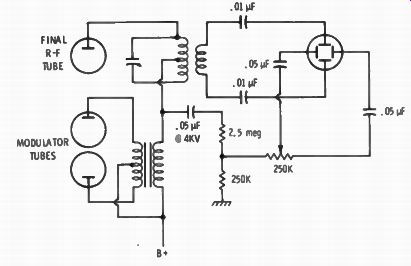
Fig. 7-25. Circuit for picking off audio from a plate modulator, using a resistor
voltage divider to reduce voltage.
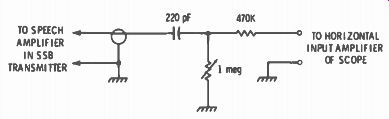
Fig. 7-26. It may be necessary to reverse the audio phase shift by using this
circuit for audio instead of the one shown in Fig. 7-24.
... but appear to be folded over, there is phase shift. In that case the connection at the scope must be made through a phase-shift network as shown in Fig. 7-24.
Fig. 7-24 shows the connection from an ssb or frequency- or phase modulated transmitter. The connection in the transmitter is made at the last point of audio. If there is DC at that point (as from the plate of an audio amplifier tube), a blocking capacitor must also be in stalled.
The phase-shift network described corrects usual phase shifting resulting from lack of wide frequency response in the modulator.
However, sometimes the shift is in the other direction. This calls for the use of the phase-shift network shown in Fig. 7-26. If one circuit does not work, change to the other.
Phase-shift networks are frequency discriminating. Adjustment of the variable resistor will correct for a single audio frequency from an audio generator. It sometimes does not correct for the random frequencies developed by the human voice. Perfect correction might involve replacing some coupling capacitors in the transmitter speech amplifier and modulator circuits. If satisfactory correction is not easily obtained, it is simpler to use the sweep circuit of the scope for your observations.
A commercial monitoring scope with built-in tuned circuits is shown in Fig. 7-27.
OBSERVING PATTERNS
Fig. 7-28 shows a series of patterns obtained from the output of an a-m transmitter. When the carrier is applied to the vertical-deflection plates and no signal or sweep voltage is applied to the horizontal plates, a bright vertical line only is seen as at A. Turn on the internal sweep generator of the scope, using any frequency of sweep, and the pattern will become a solid block as at B. The width of the pattern is arbitrary, and is adjusted to suit the observer. The height is related to the amount of r-f output from the transmitter. Pattern C is
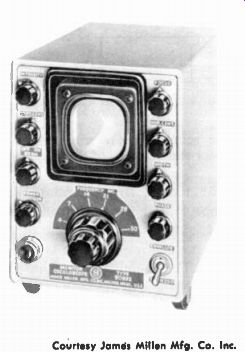
Fig. 7-27. A commercial monitoring scope with tuned circuits for vertical
deflection built in. Courtesy James Millen Mfg. Co. Inc.
what you see when you key the transmitter with a series of dots from an automatic or semiautomatic key. The sweep frequency is set at a low rate in order to synchronize with the speed of the dots to make the pattern stand still. Observe the squareness of the make and break points in the r-f squares. If the pattern is too square it means that there is no keying filter, and spurious frequencies could be created when the circuit is made and broken with the key. There should be a slight taper off the trailing end. When a single sine-wave audio frequency is fed into the microphone jack from an audio generator the pattern will look like D. This is 100-percent modulated.
If you drew lines around the edges of the pattern they should make two overlapping sine waves. If the edges are a good sine wave, the modulation quality is excellent. The sweep of pattern D is the internal sweep of the scope and, again, synchronized to the frequency injected.
If audio (voice or sine wave) is used to sweep the horizontal trace, the pattern is a trapezoid like pattern E. At 100-percent modulation you will see a perfect triangle with good sharp corners. Overmodulation will have a tip sticking out the left corner, and the top and bottom corners may begin to round out. Less than 100-percent modulation is shown in pattern F. You can measure the height of the pattern vertical sides and find percent of modulation with the following formula:
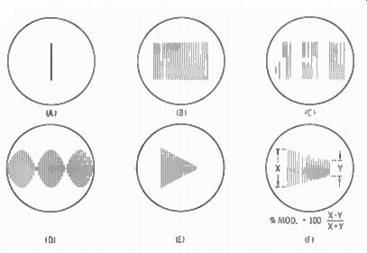
Fig.
7-28. Oscilloscope patterns obtained from a plate-modulated or c-w transmitter.
See text for explanations.
% Mod = 100 x - y / X + y
where,
X is the maximum amplitude,
y is the minimum amplitude.
SSB PATTERNS
With the ssb transmitter but with no modulation, the pattern on the scope trace will look like pattern A of Fig. 7-29-just a dot. A suppressed-carrier ssb transmitter with no modulation has no output, thus no pattern will show on the scope. Turn on the horizontal sweep for a 30-Hz sweep and the pattern will be just a horizontal line from the sweep. Modulate with voice through the microphone and it will look like pattern B. Remove the microphone and connect an audio generator. As you increase the audio input you will see a pattern like C; this is straight cw. The single audio tone has brought the carrier up to a steady state. As you increase the audio a point will be reached where the pattern height does not increase. This is maximum modulation and is the point at which "flat-topping" occurs with voice modulation. You have reached plate-current saturation in the final. Mark the top and bottom on the CRT face with a grease pencil for future reference. These will be the limits for monitoring your modulation with voice. ( Don't leave this signal on for more than 30 seconds at a time. At this point, with a steady tone, you are exceeding the plate dissipation rating of the final tube or tubes, and damage could occur.)
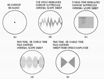
Fig. 7-29. Patterns observed on an ssb transmitter. Each pattern is described
in the text.
Parallel two audio generators with signals about 1 kHz apart and of equal level, and the pattern will look like D. This shows 100-percent modulation for an ssb transmitter if the outline of the pattern forms two sine waves overlapping and the top and bottom touches the maximum-modulation reference marks. Lacking two audio generators you can get the same pattern with one tone and carrier insertion.
With the audio off, insert carrier for a bar like pattern C but with half the height marked on the CRT with your grease pencil. Add audio to the height marked on the face of the tube. This is the equivalent to the "two-tone" signal recommended for studying linearity of the final class-B amplifier. With this setup (or the two-tone signal) switch the horizontal amplifier to direct audio from the transmitter. This will show a bow-tie pattern as shown in E. The bow-tie is actually a superior pattern for observing linearity. If the lines cross with a perfect X and the top and bottom corners are sharp, your final has good linearity and is properly loaded.
For continuous monitoring of an ssb transmitter with voice, use the internal sweep of the scope. If your voice peaks just touch the limits you have marked on the scope face, you are modulating within the limits necessary to prevent flat-topping. Your average plate current will probably be about 16 that of full c-w plate current (as for pat tern C).